On a Class of Estimation and Test for Long Memory

(1)

Munich Personal RePEc Archive

On a Class of Estimation and Test for

Long Memory

Fu, Hui

Jinan University

6 December 2012

Online at

https://mpra.ub.uni-muenchen.de/47978/

(2)

On a Class of Estimation and Test for Long Memory

Hui Fu

∗

Jinan University

Abstract: This paper advances a new analysis technology path of estimation and test for long memory time series. I propose the definitions of time scale series, strong variance scale exponent and weak variance scale exponent, and prove the strict mathematical equations that strong and weak variance scale exponent can accurately identify the time series of white noise, short memory and long memory, especially derive the equation relationships between weak variance scale exponent and long memory parameters. I also construct two statistics whichSLmemory statistic tests for long memory properties. The paper further displays Monte Carlo performance for MSE of weak variance scale exponent estimator and the empirical size and power of SLmemory statistic, giving practical recommendations of finite-sample, and also provides brief empirical examples of logarithmic return rate series data for Sino-US stock markets.

Keywords: Long Memory, Weak Variance Scale Exponent,SLmemoryStatistic, Time Scale Series. JEL Classification: C22, C13, C12.

1 Introduction and Setup

The first research of estimation for long memory dated back to Hurst (1951) who proposed classical rescaled range (R/S) method to analyze long-range dependence and subsequently refined by excellent scholars (Mandelbrot and Wallis, 1969; Mandelbrot, 1972, 1975; Mandelbrot and Taqqu, 1979; Peters, 1999, 2002). Following, fractional Gaussian noises process (Mandelbrot and Van Ness, 1968) was the first long memory model, with the long memory parameterH (Hurst exponent, also called self-similarity parameter) satisfying 0< H <1. And Lo (1991), Kwiatkowski et al. (1992) and Giraitis et al. (2003) further promote and develop the study of tests for long memory properties following the R/S-type method. Fractional differencing noises process (Granger and Joyeux, 1980; Hosking, 1981) was the second long memory model and formed the second technology path of estimation and test for long memory properties, with the long memory parameter (fractional differencing parameterd) satisfying −0.5< d < 0.5. Corresponding work include Geweke and Porter-Hudak (1983), Haslett and Raftery (1989), Beran (1994), Robinson (1995, 2005), among many others.

Lo (1991), Baillie (1996), Giraitis et al. (2003), Robinson (2003), Palma (2007) and Boutahar et al. (2007) provided relevant literature review in detail.

It is no doubt that the model parameter satisfying 0.5< H < 1, or 0< d < 0.5 is thought as long memory, long-range dependence, or persistence, and as anti-persistence for the situation of 0< H <0.5 or −0.5 < d <0. But there is argument that whether anti-persistence is long memory (Hosking, 1981;

∗_{Hui Fu is from School of Economics, Jinan University, Guangzhou, China. E-mail: fuhuicn@gmail.com or}

(3)

Lo, 1991; Palma, 2007). The present paper suggest that the situations of 0.5< H <1, 0< d <0.5 regard as persistent long memory, and as anti-persistent long memory for 0< H <0.5 or−0.5< d <0. Thus, persistent long memory means long-run positive correlation, and anti-persistent long memory implies long-run negative correlation.

The main theoretical contribution of this paper is to build a new systematic technology path for theory analysis of stationary time series, especially for the estimation and test of long memory properties. All of those the definitions of time scale series, strong variance scale exponent and weak variance scale exponent, the equation relationships between the short, long memory time series and variance scale exponents, and the two new statistics for the hypothesis tests of white noise, short memory and long memory time series, jointly form the basic components of the new technology path.

The second contribution of this paper is to show that the asymptotic properties for estimation and test can distinguish anti-persistent long memory from persistent long memory. Further it is the main reason that I advance the two types of (persistence and anti-persistence) long memory in the present paper.

The final contribution is to analyze time series properties based on the both time and frequency domain perspectives, and corresponding long memory models are confined to time and frequency domain analysis perspectives in the paper, which differs the situations that the two traditional technology paths. The plan of the paper is as follow. In sections 2 and 3, I propose the definitions of time scale series, strong variance scale exponent and weak variance scale exponent, and prove the equations between variance scale exponents and the situations that white noise, short memory and long memory time series. I also constructW noiseandSLmemorystatistics to test for white noise, short memory and long memory time series. Section 4 investigates by Monte Carlo simulations the finite-sample performance of weak variance scale exponent estimator andSLmemory statistic, giving practical recommendations for the choice of maximum time scalen. Section 5 concludes. The derivations are given in the Appendix.

I now detail the setting for the paper. Let{x(t), t= 1,2,· · · , N, N → ∞}be a stationary time series with unknown mean µand lag-i autocovarianceγi. Let the spectral density ofx(t) be denoted byf(λ)

and defined over |λ| ≤ π. d _{denotes long memory parameter of fractional differencing noises process}

(Granger and Joyeux, 1980; Hosking, 1981). H _{denotes long memory parameter of fractional Gaussian}

noises process (Mandelbrot and Van Ness, 1968). N _{denotes sample sizes.}

2 Definitions and Properties of Strong and Weak Variance Scale

Exponent

2.1 Definitions

Definition 2.1.1 Time Scale Series

For the time series {x(t)}, the new time series {x1

2=x(2t−1) +x(2t), t= 1,2,· · ·, M, M =⌊N/2⌋} and {x2

2 =x(2t) +x(2t+ 1), t= 1,2,· · · , M, M = [(N−1)/2]} can be called time scale-2 series; And, the new time series {xi+1

n , t = 1,2,· · · , M, M = ⌊(N−i)/n⌋} are called time scale-n series, where

xi+1

n =x(nt+i) +x(nt−1 +i) +· · ·+x(nt−(n−1) +i), i= 0,1,2,· · ·,(n−1),n/N → ∞, and ⌊·⌋

means round toward zero, resulting integers.

I now list four propositions arising from definition 2.1.1:

Proposition 2.1.1 Denoted D[xin+1](i = 0,1,2,· · · , n−1) are the n variances of the time scale-n

series respectively, then

D[x1

n(t)] =D[x2n(t)] =· · ·=D[xnn(t)]. (2.1.1)

(4)

In the case, I denote the nvariances of the time scale-nseries asD[xn(t)].

Proposition 2.1.2 VarianceD[xn(t)] of time scale-nseries can be expressed in terms of

D[xn(t)] =nD[x(t)] + 2 Xn

i=1(n−i)γi, n= 1,2,· · · . (2.1.2)

Proposition 2.1.3 Lag-nautocovarianceγn of the time series{x(t)} can be expressed in terms of

γn=

1

2{D[xn+1(t)]−2D[xn(t)] +D[xn−1(t)]}, (2.1.3)

whereD[x0(t)] = 0, D[x1(t)] =D[x(t)], andn= 1,2,· · ·.

Proposition 2.1.4 The sum of lag-iautocovarianceγi can be expressed in terms of

Xn

i=−nγi =n{D[xn+1(t)]−D[xn(t)]}, n= 1,2,· · ·. (2.1.4)

Definition 2.1.2 Strong Variance Scale Exponent

For the time series{x(t)}, if the variance of time scale-nseries satisfies

D[xn(t)] =n2FnD[x(t)], n= 1,2,· · ·, (2.1.5)

and ifFn equal to a constant ˙F. Thus ˙F can be called Strong Variance Scale Exponent.

Definition 2.1.3 Weak Variance Scale Exponent

For the time series{x(t)}, if the variance of time scale-nseries satisfies

D[xn(t)] =f n2FnD[x(t)], (2.1.6)

andFn get the convergence to a constantF, asn→ ∞. Thus F andf are called Weak Variance Scale

Exponent and adjusted proportion coefficient respectively.

2.2 Time Domain Analysis

Base on four propositions arising from definition 2.1.1, I obtain following results. Theorem 2.2.1 If the time series{x(t)}is white noise series, then

D[xn(t)]/D[x(t)] =n, n= 1,2,· · ·. (2.2.1)

I now list a implication arising from Theorem 2.1.1:

Proposition 2.2.1If the time series{x(t)}is white noise series, then strong variance scale exponent ˙

F, weak variance scale exponentF and adjusted proportion coefficientf satisfy:

˙

F= 0.5, F = 0.5, f= 1 (2.2.2)

respectively.

Theorem 2.2.2 If the time series{x(t)}is short memory ARMA(p,q) time series, then

D[xn(t)]/D[x(t)]∼cn, (2.2.3)

wheren→ ∞, and cis a constant.

(5)

Proposition 2.2.2 If the time series{x(t)} is short memory ARMA(p,q) series, then weak variance scale exponentF and adjusted proportion coefficientf satisfy:

F = 0.5, f = 1 (2.2.4)

respectively.

Theorem 2.2.3 If the time series{x(t)} is fractional Gaussian noises process (Mandelbrot and Van Ness, 1968), then

D[xn(t)]/D[x(t)]∼n2H, as n→ ∞, (2.2.5)

whereH is the long memory parameter of fractional Gaussian noises process.

Proposition 2.2.3If the time series{x(t)}is fractional Gaussian noises process, then weak variance scale exponentF and adjusted proportion coefficientf satisfy:

F =H, f = 1 (2.2.6)

respectively.

Theorem 2.2.4If the time series{x(t)}is fractional differencing noises process (Granger and Joyeux, 1980; Hosking, 1981, ARFIMA(0,d,0) time series), then

D[xn(t)]/D[x(t)]∼

Γ(1−d) (1 + 2d)Γ(1 +d)n

1+2d_{, as n}

→ ∞, (2.2.7)

wheredis the long memory parameter of fractional differencing noises process and Γ(·) denotes Gamma function.

Proposition 2.2.4If the time series{x(t)}is fractional differencing noises process, then weak variance scale exponentF and adjusted proportion coefficientf satisfy:

F =d+ 0.5, f = Γ(1−d)

(1 + 2d)Γ(1 +d) (2.2.8)

respectively.

2.3 Frequency Domain Analysis

For the stationary time series{x(t)}, if the autocovarianceγiis absolutely summable, then the spectral

densityf(λ) satisfy:

f(λ) = 1 2π

X∞

k=−∞γke

−ikλ₌ 1

2π

X∞

k=−∞γkcos(kλ). (2.3.1)

setλ= 0, then

f(λ= 0) = 1 2π

X∞

k=−∞γk. (2.3.2)

Based on Proposition 2.1.2, I obtain following results.

Theorem 2.3.1 If the time series{x(t)}is white noise series, then

D[xn(t)] = 2nπf(0), n= 1,2,· · ·. (2.3.3)

Theorem 2.3.2 If the time series{x(t)}is short memory ARMA(p,q) series, then

D[xn(t)]∼2nπf(0), as n→ ∞. (2.3.4)

(6)

Proposition 2.2.1 and Proposition 2.2.2 can also arising from Theorem 2.3.1 and Theorem 2.3.2 respec-tively.

It need to be pointed out that the autocovariance of stationary long memory time series is not abso-lutely summable, but the generalized relationship theorem for a stationary time series between spectral densityf(λ) and varianceD[xn(t)] of time scale-nseries is display as following:

Theorem 2.3.3 For the stationary time series{x(t)}, then

D[xn(t)] = 2 Z π

−π

f(λ)1−cos(nλ)

[2sin(λ/2)]2dλ, n= 1,2,· · · . (2.3.5)

Obviously, Theorem 2.3.3 is the generalization of Theorem 2.3.1 and Theorem 2.3.2. Arising from Theo-rem 2.3.3, I educe TheoTheo-rem 2.3.4:

Theorem 2.3.4 If the time series{x(t)}is generalized ARFIMA(p,d,q) series, then

D[xn(t);p, d, q]/D[x(t)]∼c(φ, θ)

Γ(1−d) (1 + 2d)Γ(1 +d)n

1+2d_{, as n}

→ ∞. (2.3.6)

In which, c(φ, θ) is a constant. And if p=q ≡0, thenc(φ, θ) = 1; otherwise, c(φ, θ)∈[c1,1)∪(1, c2],

c1=

min_{|θ(1)|2_,_|_θ₍₋₁₎_|2_}

max{|φ(1)|2_,_|_φ₍₋₁₎_|2_} andc2=

max_{|θ(1)|2_,_|_θ₍₋₁₎_|2_}

min{|φ(1)|2_,_|_φ₍₋₁₎_|2_}.

I now list a implication arising from Theorem 2.3.4:

Proposition 2.3.1 If the time series {x(t)} is generalized ARFIMA(p,d,q) time series, then weak variance scale exponentF and adjusted proportion coefficient f satisfy:

F =d+ 0.5, f =c(φ, θ) Γ(1−d)

(1 + 2d)Γ(1 +d) (2.3.7)

respectively.

3 Hypothesis Tests

3.1 Wnoise

Statistic

I construct two hypothesis test statistics to analyze the memory properties considering white noise, short memory and long memory time series.

If the stationary time series {x(t), t= 1,2, . . .} is independent white noise series, as n→ ∞, apply Lindbergh Central Limit Theorem, then

√

nXn

t=1x(t)/n −µ

_d

−→N(0, D[x(t)]), (3.1.1)

and

xn(t)−nµ p

nD[x(t)]

d

−→N(0,1). (3.1.2)

where −→d denotes convergence in distribution. Denotes ˆD[x(t)] as sample variance, based on Slutsky Theorem, then

xn(t)−nPNt=1x(t)/N

q

nDˆ[x(t)]

d −

(7)

and

(N(n)−1)Dˆ[xn(t)] nDˆ[x(t)]

d −

→χ2(N(n)−1), (3.1.4)

whereN(n) denotes the time series{xn(t)} sample sizes.

Denote

W noise(n) = (N(n)−1)Dˆ[xn(t)]

nDˆ[x(t)]. (3.1.5)

W noisestatistic tests under independent white noise hypotheses and non-independent stochastic process alternatives.

3.2 SLmemory

Statistic

As a generalization situation, if the stationary time series{x(t), t= 1,2,· · · }is short memory series and apply central limit theorem(Anderson, 1971, Theorem 7.7.8; Brockwell and Davis, 1991, Theorem 7.1.2), then

√

nXn

t=1x(t)/n −µ

_d

−→N(0,X∞

i=−∞γi), as n→ ∞. (3.2.1) Based on Slutsky Theorem and Proposition 2.1.4, I educe the following conclusion:

xn(t)−nPNt=1x(t)/N

q

n( ˆD[xn+1(t)]−Dˆ[xn(t)]) d

−→N(0,1). (3.2.2)

Then

(N(n)−1) ˆD[xn(t)]

nDˆ[xn+1(t)]−Dˆ[xn(t)]

d

−→χ2(N(n)−1). (3.2.3)

Denote

SLmemory(n) = (N(n)−1) ˆD[xn(t)] nDˆ[xn+1(t)]−Dˆ[xn(t)]

. (3.2.4)

SLmemorystatistic tests under white noise, short memory null hypotheses and long memory alternatives. Obviously,SLmemory statistic is a monotonic decreasing function of long memory parameterd.

Further, if the alternatives are limited in the situation of anti-persistent long memory, the two classical long memory parameters satisfies−0.5< d <0, 0< H <0.5 respectively, the reject region of hypothesis test ofSLmemory statistic is:

SLmemory(n)≥χ21−α(N(n)−1) , (3.2.5)

whereαis significance size.

And if the alternatives are limited in the situation of persistent long memory, two classical long memory parameters satisfies 0< d <0.5, 0.5< H <1 respectively, the reject region of hypothesis test ofSLmemory statistic is:

SLmemory(n)≤χ2α(N(n)−1) . (3.2.6)

(8)

4 Monte Carlo Performance

The objective of this section is to illustrate the asymptotic properties for weak variance scale exponent estimator and SLmemory statistic, to examine their finite-sample performance, and to give advice on how to choose the time scale n in practical applications. I focus on the MSE for weak variance scale exponent estimator and the empirical size and power forSLmemorystatistic. Throughout the simulation exercise, the number of replications is 1000.

4.1 Monte Carlo Study for Weak Variance Scale Exponent Estimator

Based on the definition of weak variance scale exponent, it can be transferred to:

y(i) =f[z(i)]F, (4.1.1)

where y(i) = D[xi(t)]/D[x(t)],z(i) =i2,i = 1,2,· · ·, n. n is the maximum time scale of finite-sample

series. Estimate the parameterF in non-linear regression by sample series{y(i)} and {z(i)}, then gain the weak variance scale exponent estimator ˆF.

Let stationary time series{x(t)}be a linear generalized Gaussian ARFIMA (1,d_{,1) process (1}₋_φB₎₍₁₋

B)d_X

t = (1−θB)εt, with unit standard deviation, for different values of φ, θ and d. I consider four

sample sizesN=250, 500, 1000, 2000, and estimate the parameterdusing weak variance scale exponent with maximum time scalen=⌊Nm⌋, wheremare the 13 numbers which range from 0.2 to 0.8 and step length by 0.05.

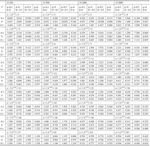
Table 1 contains the MSE of the weak variance scale exponent estimator calculated for different values of maximum time scale n =⌊Nm_⌋_{. When} _φ ₆_{= 0, or} _θ ₆_{= 0, the MSE show approximate U-type curve}

shape, and when d =φ =θ=0, the MSE increase slowly. Generally, m=0.5 and n =⌊N0.5_⌋_{could be} optimal choice of weak variance scale exponent estimator in practice.

4.2 Monte Carlo Study for

SLmemory

Statistic

The Monte Carlo study for SLmemory statistic investigate the percentage of replications in which the rejection of a short memory (or white noise) null hypothesis was observed. Thus if a data generating process belongs to the null hypothesis, the empirical test sizes will be calculated. And if it is a long memory process, the empirical power of the tests will be provided.

Let stationary time series{x(t)} be a linear ARMA(1,1) model (1−φB)Xt= (1−θB)εt, with unit

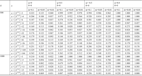
standard deviation, for different values ofφandθ. I consider two sample sizesN=500, 1000, and choose time scalen=⌊Nm_⌋_,_m _{are the 13 numbers which are from 0.2 to 0.8 and step length is 0.05. Table 2}

display empirical size of ARMA(1,1) model for the situations of different time scalen=⌊N0.4_⌋_{. Table 2} shows that, asmincrease, empirical size show approximate U-type curve shape.

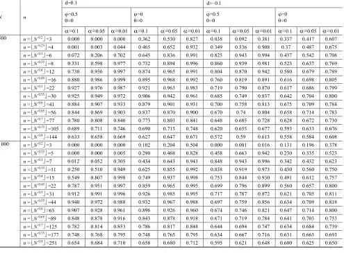
Table 3 compares the power of the tests under long memory alternatives. I consider the long memory ARFIMA (1,d,1) model (1−φB)(1−B)d_X

t = (1−θB)εt, with unit standard deviation, for different

values ofφ,θandd, and for two sample sizesN=500, 1000. In table 3, whilemincrease, empirical power show approximate inverse U-type curve shape, and obviously contrast to the situation of Table 2.

(9)

[image:9.612.61.558.164.648.2]

Table 1

MSE (in %) of weak variance scale exponent estimator. Let stationary time series {x(t)} be a linear generalized Gaussian ARFIMA(1, d, 1) process (1－B)(1－B)dXt=(1－B)t , with unit standard deviation, for different values of ,  and d, and N denotes sample sizes.

d

N=250 N=500 N=1000 N=2000

=0.5

=0

=0

=-0.5 =0.5

=-0.5 =0

=0

=0.5

=0

=0

=-0.5 =0.5

=-0.5 =0

=0

=0.5

=0

=0

=-0.5 =0.5

=-0.5 =0

=0

=0.5

=0

=0

=-0.5 =0.5

=-0.5 =0

=0

n = N 0.2_₌₃ _n₌__N0.2_₌₃ _n₌__N0.2_₌₃ _n₌__N0.2_₌₄

-0.1 9.645 4.319 15.201 0.287 9.511 4.296 15.222 0.167 9.524 4.232 15.162 0.117 7.740 2.564 11.493 0.082 0 6.817 2.648 10.685 0.216 6.832 2.621 10.693 0.106 6.833 2.598 10.690 0.048 5.488 1.490 8.050 0.027

0.1 4.484 1.431 6.847 0.274 4.496 1.460 6.936 0.164 4.555 1.447 6.957 0.096 3.612 0.784 5.200 0.056

n = N 0.25_₌₃ _n₌__N0.25_₌₄ _n₌__N0.25_₌₅ _n₌__N0.25_₌₆

-0.1 9.645 4.319 15.201 0.287 7.772 2.655 11.556 0.165 6.354 1.769 9.010 0.101 5.247 1.298 7.260 0.068

0 6.817 2.648 10.685 0.216 5.475 1.532 8.038 0.123 4.410 0.990 6.230 0.063 3.604 0.691 4.962 0.036

0.1 4.484 1.431 6.847 0.274 3.538 0.809 5.140 0.171 2.832 0.487 3.942 0.092 2.288 0.332 3.115 0.055

n = N 0.3_₌₅ _n₌__N0.3_₌₆ _n₌__N0.3_₌₇ _n₌__N0.3_₌₉

-0.1 6.536 1.936 9.112 0.317 5.337 1.414 7.357 0.184 4.415 1.036 5.972 0.100 3.215 0.688 4.241 0.065 0 4.443 1.139 6.244 0.277 3.635 0.784 4.982 0.164 2.973 0.552 4.015 0.086 2.107 0.344 2.776 0.052

0.1 2.792 0.576 3.836 0.357 2.245 0.401 3.071 0.212 1.828 0.265 2.455 0.110 1.265 0.161 1.657 0.065

n = N 0.35_₌₆ _n₌__N0.35_₌₈ _n₌__N0.35_₌₁₁ _n₌__N0.35_₌₁₄

-0.1 5.473 1.525 7.395 0.343 3.873 0.974 5.141 0.212 2.490 0.565 3.213 0.126 1.740 0.381 2.214 0.080

0 3.656 0.911 4.984 0.323 2.553 0.544 3.366 0.207 1.583 0.306 2.036 0.128 1.066 0.193 1.353 0.077

0.1 2.243 0.481 2.992 0.407 1.515 0.309 2.004 0.258 0.906 0.174 1.165 0.155 0.593 0.112 0.748 0.093

n = N 0.4 =9 n = N 0.4 =12 n = N 0.4 =15 n = N 0.4 =20

-0.1 3.520 1.010 4.461 0.431 2.390 0.679 3.015 0.280 1.643 0.419 2.064 0.153 1.048 0.269 1.295 0.101 0 2.266 0.689 2.903 0.453 1.502 0.429 1.877 0.298 1.001 0.256 1.246 0.167 0.611 0.157 0.751 0.106

0.1 1.329 0.462 1.631 0.557 0.857 0.320 1.060 0.356 0.555 0.180 0.686 0.194 0.333 0.121 0.397 0.125

n = N 0.45_₌₁₁ _n₌__N0.45_₌₁₆ _n₌__N0.45_₌₂₂ _n₌__N0.45_₌₃₀

-0.1 2.823 0.883 3.447 0.488 1.690 0.592 2.072 0.343 1.016 0.348 1.242 0.198 0.645 0.228 0.758 0.138

0 1.823 0.679 2.251 0.536 1.074 0.451 1.282 0.391 0.625 0.270 0.736 0.234 0.382 0.180 0.442 0.160

0.1 1.067 0.519 1.228 0.652 0.627 0.392 0.723 0.457 0.372 0.241 0.420 0.271 0.235 0.169 0.255 0.178

n = N 0.5 =15 n = N 0.5 =22 n = N 0.5 =31 n = N 0.5 =44

-0.1 2.098 0.826 2.406 0.619 1.223 0.570 1.439 0.426 0.756 0.367 0.882 0.268 0.478 0.243 0.528 0.192 0 1.438 0.772 1.660 0.714 0.851 0.551 0.958 0.528 0.509 0.336 0.562 0.321 0.327 0.241 0.352 0.237

0.1 0.924 0.716 0.948 0.875 0.582 0.530 0.606 0.614 0.385 0.348 0.388 0.389 0.254 0.249 0.260 0.258

n = N 0.55_₌₂₀ _n₌__N0.55_₌₃₀ _n₌__N0.55_₌₄₄ _n₌__N0.55_₌₆₅

-0.1 1.760 0.926 1.918 0.805 1.040 0.643 1.170 0.560 0.672 0.448 0.749 0.382 0.435 0.311 0.463 0.278 0 1.367 0.978 1.485 0.959 0.839 0.724 0.894 0.714 0.538 0.472 0.562 0.468 0.377 0.350 0.387 0.353

0.1 1.084 1.041 1.018 1.232 0.744 0.760 0.719 0.865 0.493 0.513 0.492 0.547 0.370 0.386 0.366 0.400

n = N 0.6_₌₂₇ _n₌__N0.6_₌₄₁ _n₌__N0.6_₌₆₃ _n₌__N0.6_₌₉₅

-0.1 1.739 1.179 1.787 1.130 1.115 0.836 1.155 0.800 0.703 0.599 0.778 0.535 0.520 0.429 0.517 0.423

0 1.540 1.335 1.599 1.331 1.023 0.982 1.051 0.979 0.696 0.701 0.706 0.703 0.514 0.508 0.521 0.514

0.1 1.503 1.541 1.379 1.758 1.091 1.140 1.043 1.239 0.723 0.777 0.731 0.795 0.594 0.592 0.568 0.624

(10)

[image:10.612.57.556.134.375.2]

Table 1(continued)

MSE (in %) of weak variance scale exponent estimator.

d

N=250 N=500 N=1000 N=2000

=0.5

=0

=0

=-0.5

=0.5

=-0.5

=0

=0

=0.5

=0

=0

=-0.5

=0.5

=-0.5

=0

=0

=0.5

=0

=0

=-0.5

=0.5

=-0.5

=0

=0

=0.5

=0

=0

=-0.5

=0.5

=-0.5

=0

=0

n =N 0.65_₌₃₆ _n₌__N0.65_₌₅₆ _n₌__N0.65_₌₈₉ _n₌__N0.65_₌₁₃₉

-0.1 1.969 1.566 1.959 1.544 1.343 1.162 1.361 1.121 0.899 0.829 0.941 0.794 0.695 0.603 0.654 0.629

0 1.888 1.818 1.917 1.817 1.378 1.402 1.393 1.399 0.986 1.035 0.991 1.037 0.757 0.778 0.757 0.783

0.1 2.145 2.207 1.996 2.415 1.580 1.697 1.583 1.724 1.164 1.198 1.146 1.236 0.922 0.909 0.893 0.952

n = N 0.7 =47 n = N 0.7 =77 n = N 0.7 =125 n = N 0.7 =204

-0.1 2.394 2.091 2.383 2.062 1.781 1.639 1.791 1.604 1.348 1.219 1.300 1.260 0.995 0.962 1.000 0.948 0 2.480 2.425 2.498 2.426 1.967 2.021 1.974 2.019 1.476 1.586 1.477 1.589 1.130 1.166 1.129 1.171

0.1 2.971 3.116 2.920 3.226 2.335 2.376 2.274 2.464 1.909 1.853 1.805 1.971 1.452 1.491 1.476 1.479

n = N 0.75_₌₆₂ _n₌__N0.75_₌₁₀₅ _n₌__N0.75_₌₁₇₇ _n₌__N0.75_₌₂₉₉

-0.1 3.158 2.923 3.193 2.852 2.489 2.321 2.449 2.324 1.952 1.885 1.959 1.870 1.545 1.551 1.571 1.501

0 3.535 3.427 3.547 3.419 2.786 2.872 2.787 2.871 2.305 2.411 2.300 2.416 1.774 1.753 1.770 1.764

0.1 4.257 4.406 4.251 4.457 3.471 3.327 3.237 3.583 2.806 2.866 2.835 2.862 2.375 2.389 2.358 2.365

n = N 0.8 =82 n = N 0.8 =144 n = N 0.8 =251 n = N 0.8 =437

-0.1 4.722 4.286 4.560 4.338 3.600 3.398 3.523 3.434 2.985 2.841 2.917 2.891 2.491 2.502 2.511 2.454 0 5.501 4.992 5.539 4.971 4.227 4.438 4.225 4.428 3.453 3.592 3.449 3.599 2.723 2.716 2.755 2.775

0.1 6.447 6.159 6.025 6.567 5.274 4.931 4.851 5.373 4.344 4.182 4.130 4.367 3.625 3.776 3.822 3.699

Table 2

Empirical test sizes (in %) of SLmemory statistic of time series under the null hypothesis of ARMA(1, 1) model, (1－B) Xt=(1－B)t,

with standard normal innovations.

N n

=0

=0

=0.5

=0

=-0.5 =0

=0.8

=0

=0.1 =0.05 =0.01 =0.1 =0.05 =0.01 =0.1 =0.05 =0.01 =0.1 =0.05 =0.01 500 n = N 0.2_₌₃ _0.223 _0.123 _0.040 _0.999 _0.995 _0.978 _0.994 _0.986 _0.962 _1.000 _1.000 _1.000

n = N 0.25 =4 0.204 0.108 0.037 0.973 0.922 0.564 0.520 0.414 0.285 1.000 1.000 1.000

n = N 0.3 =6 0.187 0.101 0.037 0.578 0.336 0.028 0.501 0.405 0.257 1.000 1.000 0.981

n = N 0.35_₌₈ _0.167 _0.106 _0.041 _0.261 _0.076 _0.003 _0.431 _0.338 _0.226 _0.989 _0.947 _0.457

n = N 0.4 =12 0.169 0.115 0.048 0.100 0.028 0.009 0.357 0.272 0.164 0.655 0.275 0.000

n = N 0.45_₌₁₆ _0.180 _0.120 _0.062 _0.103 _0.053 _0.027 _0.292 _0.220 _0.122 _0.224 _0.024 _0.001

n = N 0.5_₌₂₂ _0.176 _0.122 _0.067 _0.106 _0.071 _0.037 _0.248 _0.199 _0.137 _0.063 _0.023 _0.006

n = N 0.55 =30 0.179 0.143 0.093 0.144 0.103 0.074 0.239 0.187 0.124 0.082 0.056 0.026

n = N 0.6_₌₄₁ _0.199 _0.168 _0.115 _0.169 _0.139 _0.091 _0.239 _0.184 _0.138 _0.119 _0.089 _0.059

n = N 0.65_₌₅₆ _0.231 _0.186 _0.150 _0.248 _0.197 _0.148 _0.264 _0.218 _0.179 _0.194 _0.170 _0.132

n = N 0.7 =77 0.251 0.217 0.178 0.265 0.225 0.189 0.286 0.254 0.205 0.248 0.213 0.176

n = N 0.75_₌₁₀₅ _0.329 _0.300 _0.277 _0.317 _0.288 _0.266 _0.336 _0.309 _0.279 _0.322 _0.292 _0.254

n = N 0.8_₌₁₄₄ _0.363 _0.345 _0.318 _0.363 _0.338 _0.312 _0.363 _0.348 _0.321 _0.373 _0.356 _0.339

1000 _n₌__N0.2_

=3 0.210 0.102 0.022 1.000 1.000 1.000 1.000 1.000 0.997 1.000 1.000 1.000

n = N 0.25_₌₅ _0.179 _0.094 _0.028 _0.982 _0.941 _0.667 _0.862 _0.816 _0.700 _1.000 _1.000 _1.000

n = N 0.3_₌₇ _0.150 _0.082 _0.024 _0.679 _0.476 _0.094 _0.613 _0.516 _0.358 _1.000 _1.000 _1.000

n = N 0.35 =11 0.144 0.075 0.028 0.221 0.068 0.003 0.395 0.298 0.172 0.989 0.944 0.505

[image:10.612.60.557.407.674.2]

(11)

[image:11.612.57.557.147.270.2]

Table 2(continued)

Empirical test sizes (in %) of SLmemory statistic of time series under the null hypothesis of ARMA(1, 1) model, (1－B) Xt=(1－B)t,

with standard normal innovations.

N n

=0

=0

=0.5

=0

=-0.5 =0

=0.8

=0

=0.1 =0.05 =0.01 =0.1 =0.05 =0.01 =0.1 =0.05 =0.01 =0.1 =0.05 =0.01 1000 _n₌__N0.5_

=31 0.157 0.091 0.046 0.106 0.064 0.026 0.240 0.166 0.090 0.082 0.025 0.012

n = N 0.55_₌₄₄ _0.172 _0.128 _0.060 _0.142 _0.098 _0.044 _0.213 _0.153 _0.096 _0.085 _0.059 _0.032

n = N 0.6_₌₆₃ _0.196 _0.143 _0.089 _0.156 _0.119 _0.070 _0.204 _0.154 _0.093 _0.138 _0.100 _0.063

n = N 0.65 =89 0.234 0.193 0.132 0.217 0.169 0.129 0.251 0.206 0.143 0.170 0.143 0.110

n = N 0.7_₌₁₂₅ _0.267 _0.239 _0.191 _0.285 _0.244 _0.188 _0.296 _0.248 _0.196 _0.231 _0.193 _0.150

n = N 0.75_₌₁₇₇ _0.322 _0.285 _0.243 _0.304 _0.275 _0.240 _0.317 _0.288 _0.251 _0.284 _0.255 _0.217

n = N 0.8 =251 0.383 0.355 0.322 0.376 0.349 0.329 0.390 0.362 0.332 0.373 0.346 0.322

Table 3

Empirical power of the tests (in %) based on SLmemory statistic, the alternatives considered are ARFIMA(1, d, 1) model, (1－B)(1－ B)dXt=(1－B)t, with standard normal innovations.

N n

d=0.1 d=-0.1

=0.5

=0

=0

=0

=0.5

=0

=0

=0

=0.1 =0.05 =0.01 =0.1 =0.05 =0.01 =0.1 =0.05 =0.01 =0.1 =0.05 =0.01 500 n = N 0.2_₌₃ _0.000 _0.000 _0.000 _0.362 _0.530 _0.827 _0.038 _0.092 _0.381 _0.337 _0.417 _0.607

n = N 0.25_₌₄ _0.001 _0.003 _0.044 _0.465 _0.652 _0.932 _0.349 _0.536 _0.908 _0.37 _0.487 _0.675

n = N 0.3 =6 0.072 0.206 0.702 0.645 0.836 0.991 0.825 0.943 0.994 0.437 0.542 0.708

n = N 0.35_₌₈ _0.331 _0.598 _0.977 _0.732 _0.894 _0.996 _0.860 _0.939 _0.981 _0.523 _0.637 _0.769

n = N 0.4_₌₁₂ _0.730 _0.936 _0.997 _0.874 _0.965 _0.991 _0.804 _0.870 _0.942 _0.580 _0.679 _0.789

n = N 0.45 =16 0.880 0.986 0.999 0.895 0.968 0.992 0.760 0.819 0.891 0.616 0.698 0.805

n = N 0.5_₌₂₂ _0.927 _0.976 _0.987 _0.921 _0.963 _0.983 _0.719 _0.790 _0.870 _0.617 _0.686 _0.799

n = N 0.55_₌₃₀ _0.925 _0.949 _0.972 _0.906 _0.942 _0.961 _0.685 _0.749 _0.837 _0.642 _0.704 _0.800

n = N 0.6 =41 0.884 0.907 0.933 0.879 0.901 0.931 0.700 0.758 0.813 0.675 0.709 0.784

n = N 0.65_₌₅₆ _0.844 _0.869 _0.903 _0.837 _0.870 _0.900 _0.670 _0.74 _0.804 _0.658 _0.714 _0.783

n = N 0.7_₌₇₇ _0.780 _0.808 _0.840 _0.773 _0.803 _0.841 _0.648 _0.685 _0.728 _0.628 _0.672 _0.730

n = N 0.75 =105 0.689 0.711 0.746 0.690 0.715 0.748 0.620 0.655 0.677 0.593 0.633 0.676

n = N 0.8_₌₁₄₄ _0.633 _0.658 _0.669 _0.627 _0.647 _0.671 _0.572 _0.59 _0.613 _0.558 _0.584 _0.608

1000 n = N 0.2 =3 0.000 0.000 0.000 0.102 0.204 0.504 0.000 0.001 0.016 0.131 0.196 0.378

n = N 0.25 =5 0.000 0.000 0.005 0.290 0.468 0.828 0.458 0.663 0.942 0.230 0.335 0.523

n = N 0.3_₌₇ _0.012 _0.052 _0.305 _0.434 _0.643 _0.943 _0.848 _0.943 _0.996 _0.342 _0.432 _0.623

n = N 0.35 =11 0.250 0.510 0.949 0.625 0.855 0.992 0.838 0.919 0.973 0.430 0.560 0.750

n = N 0.4_₌₁₅ _0.549 _0.807 _0.998 _0.749 _0.937 _0.998 _0.753 _0.844 _0.930 _0.491 _0.612 _0.757

n = N 0.45_₌₂₂ _0.787 _0.951 _0.997 _0.859 _0.965 _0.995 _0.699 _0.796 _0.899 _0.560 _0.657 _0.800

n = N 0.5 =31 0.912 0.991 0.996 0.926 0.985 0.995 0.717 0.787 0.872 0.621 0.705 0.811

n = N 0.55_₌₄₄ _0.940 _0.972 _0.988 _0.932 _0.967 _0.988 _0.697 _0.759 _0.856 _0.634 _0.709 _0.818

n = N 0.6_₌₆₃ _0.907 _0.928 _0.961 _0.896 _0.926 _0.960 _0.674 _0.746 _0.821 _0.647 _0.714 _0.800

n = N 0.65 =89 0.848 0.878 0.916 0.843 0.878 0.918 0.671 0.719 0.784 0.641 0.703 0.753

n = N 0.7_₌₁₂₅ _0.782 _0.814 _0.853 _0.786 _0.817 _0.848 _0.644 _0.694 _0.747 _0.634 _0.684 _0.739

n = N 0.75_₌₁₇₇ _0.748 _0.768 _0.795 _0.748 _0.765 _0.795 _0.634 _0.667 _0.716 _0.631 _0.663 _0.693

n = N 0.8 =251 0.654 0.684 0.710 0.658 0.680 0.712 0.595 0.621 0.648 0.600 0.625 0.650

[image:11.612.63.558.308.673.2]

(12)

4.3 Application to Sino-US Stock Index Return Rate Data

[image:12.612.93.505.245.326.2]

I illustrate the theory and simulations by applying the weak variance scale exponent estimator and SLmemorystatistic to the logarithmic return rate data of Sino-US stock index. To make the results com-parable with the simulations, I divide each logarithmic return rate series into three blocks of approximate lengths (about 1000) as shown in table 4.

Table 4

Descriptive Statistics. CN. and US. Block denotes Shanghai Composite and Standard & Poor 500 index data respectively. Block 1 is for a period of four years from January 1, 2000 to December 31, 2003. Block 2 is also for a period of four years from January 1, 2004 to December 31, 2007. Block 3 ranges a period from January 1, 2008 to May 25, 2012.

Sample Sizes Mean Std.Dev Minimum Maximum Skewness Kurtosis CN.Block 1 957 0.0095 1.3666 -6.5437 9.4014 0.7929 7.5504 CN.Block 2 968 0.1298 1.6209 -9.2562 7.8903 -0.4333 3.1152 CN.Block 3 1069 -0.0761 1.9062 -8.0437 9.0348 -0.1541 2.8143 US.Block 1 1004 -0.0278 1.3814 -6.0045 5.5744 0.1447 1.2812 US.Block 2 1006 0.0276 0.7612 -3.5343 2.8790 -0.3088 1.7889 US.Block 3 1110 -0.0097 1.7393 -9.4695 10.9572 -0.2300 6.3233

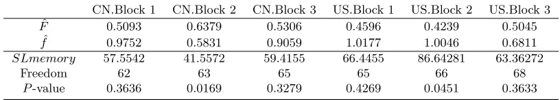
The weak variance exponent estimators, the SLmemorystatistic values and correspondingP-values are displayed in table 5. The evidence against the null hypothesis in favor of long memory alternative is strong for the second blocks of Sino-US stock index series which the weak variance exponent estimators are 0.6379, 0.4239 respectively. The first and third blocks of Sino-US stock index series show that their weak variance exponent estimators are all close to 0.5 and the corresponding P-values are all beyond 0.3, that it is inclined to believe that the data exhibit some forms of accepting the null hypothesis discussed in the present paper. In a word, the weak variance exponent estimators are consist with statistical tests for Sino-US stock index series and the results show that there is long memory in Sino-US stock index series for the period that from January 1, 2004 to December 31, 2007, and no long memory in Sino-US stock index series for the other two periods.

Table 5

Estimation and Test Results for Sino-US Stock Index Data.

CN.Block 1 CN.Block 2 CN.Block 3 US.Block 1 US.Block 2 US.Block 3 ˆ

F 0.5093 0.6379 0.5306 0.4596 0.4239 0.5045 ˆ

f 0.9752 0.5831 0.9059 1.0177 1.0046 0.6811

SLmemory 57.5542 41.5572 59.4155 66.4455 86.64281 63.36272

Freedom 62 63 65 65 66 68

P-value 0.3636 0.0169 0.3279 0.4269 0.0451 0.3633

[image:12.612.94.502.506.579.2]

(13)

for anti-persistence. The economics meanings for the periods of Block 2 can be interpret that Shanghai stock market was more vulnerable to the impact of external events and it lasted for a long time, while Standard & Poor stock market can quickly return to stability under the influence of external shocks.

5 Conclusions

The goal of this paper is to introduce a new system standpoint for theory analysis of stationary time series, especially for long memory properties, referring to estimation and test for long memory properties in the present paper. Combining with both time and frequency domain analysis, the properties of strong and weak variance scale exponent of white noise, short memory ARMA(p,q) and long memory ARFIMA(p,d,q) time series have been derived. And particularly conclude the equations between weak variance scale exponent and long memory parameter d(−0.5 < d < 0.5), H(0 < H < 1). Further, under independent white noise null hypotheses and non-independent stochastic process alternatives, and under white noise, short memory null hypothesis and long memory alternatives, I construct W noise andSLmemory statistic tests respectively. The estimation and test allow for the possibility of memory properties of persistence or anti-persistence in theory which differ V/S statistic tests (Giraitis et al., 2003, 2005) only for persistence situations.

A Monte Carlo study for weak variance scale exponent and SLmemory statistic both refer to the selection of maximum time scalenof finite-sample. By minimizing the MSE for estimation and optimizing empirical size and power for tests, finally find thatn=⌊N0.5_⌋_{for weak variance scale exponent estimator} andn=⌊N0.4_⌋_for_SLmemory _{statistic test can be recommended in practice. In fact, time scale}_n_can also be regarded as an analogy of bandwidth (Abadir et al., 2009).

Further study of the present paper, maybe consider that, to analyze the properties of strong and weak variance scale exponent for non-stationary or non-invertibility time series, more complicated long memory model and corresponding statistical tests. Surely, on estimation of autocovariance, proposition 2.1.3 can be considered as a replacement of Durbin-Levinson algorithm.

Acknowledgments

This paper is mainly based on chapter 4 and 5 of my dissertation at Yunnan University of Finance and Economics. And the research was partially supported by the Yunnan University of Finance and Economics Graduate Student Innovation Project grant YFGI(2011)019. I am grateful to my supervisor Professor Guoqing Zhao for leading me interested in the topic of long memory time series and giving me important guidances. I also thank Yunnan University of Finance and Economics Professor Peng Bai for useful helps during my studying on the topic and the constructive comments during my thesis defense.

Appendix. Proofs of The Theorems and An Auxiliary Lemma

Proof of Theorem 2.2.2 Proposition 2.1.2 can rewrite

D[xn(t)] = Xn

i=−n(n−i)γi=nγ0 Xn

i=−nρi− Xn

i=−niγi. (A.1)

For the short memory time series, the cumulant of autocorrelation ρi convergence

lim

n→∞

Xn

−nρi →c, (A.2)

(14)

wherec_{is a constant. And under the condition of short memory time series, applying Kronecker lemma:}

1 n

Xn

i=1iγi →0, as n→ ∞. (A.3)

to complete the proof of Theorem 2.2.2.

Proof of Theorem 2.2.3The Lag-nautocovarianceγnof fractional Gaussian noises process{x(t)}

satisfies:

γn=

γ0 2

h

(n+ 1)2H−2n2H+ (n−1)2Hi, as n→ ∞. (A.4)

Using proposition 2.1.3,

γn =

1

2{D[xn+1(t)]−2D[xn(t)] +D[xn−1(t)]}, n= 1,2,· · ·. (A.5) I obtain

D[xn(t)]/D[x(t)]∼n2H, as n→ ∞. (A.6)

D[xn(t)] =nγ0+ 2γ0

h

(n+d)Xn

k=1ρk−

Xn

k=1(k+d)ρk

i

. (A.7)

DenoteS1(n) =Pn_k₌₁ρk, S2(n) =Pn_k₌₁(k+d)ρk respectively, that

S1(n) =

Xn k=1ρk

= d

1−d+

d(1 +d)

(1−d)(2−d)+· · ·+

d(1 +d)· · ·(n−1 +d) (1−d)(2−d)· · ·(n−d)

= 1

2

_{1 +}_d

1−d−1

+1 2

1 +d 1−d

_{2 +}_d

2−d−1

+· · ·+

1 2

(1 +d)(2 +d)· · ·(n−1 +d) (1−d)(2−d)· · ·(n−1−d)

₍_n₊_d₎

(n−d)−1

=−1

2 +

1 2

Γ(1−d)Γ(n+ 1 +d) Γ(1 +d)Γ(n+ 1−d),

(A.8)

and

S2(n) =

Xn

k=1(k+d)ρk

=d

1 +d 1−d+

(1 +d)(2 +d)

(1−d)(2−d)+· · ·+

(1 +d)(2 +d)· · ·(n−1 +d)(n+d) (1−d)(2−d)· · ·(n−1−d)(n−d)

=d1 +d 1 + 2d

2 +d 1−d−1

+d1 +d 1 + 2d

(2 +d)(3 +d) (1−d)(2−d)−

(2 +d) (1−d)

+· · ·+

d1 +d 1 + 2d

_{(2 +}_d_{)(3 +}_d₎

· · ·(n+d)(n+ 1 +d) (1−d)(2−d)· · ·(n−1−d)(n−d)−

(2 +d)(3 +d)· · ·(n+d)(n−d) (1−d)(2−d)· · ·(n−1−d)(n−d)

=d

−1 +d

1 + 2d+ 1 1 + 2d

Γ(1−d)Γ(n+ 2 +d) Γ(1 +d)Γ(n+ 1−d)

.

(15)

Then

D[xn(t)] =γ0

_d

1 + 2d+ 1 1 + 2d

Γ(1−d)Γ(n+ 1 +d) Γ(1 +d)Γ(n−d)

. (A.10)

By Stirling formula: Γ(x)∼√2πe1−x₍_x₋₁₎x−1/2

, as x→ ∞. Therefore

D[xn(t)]/D[x(t)]∼

1 1 + 2d

Γ(1−d) Γ(1 +d)n

1+2d_,

−1/2< d <1/2, n→ ∞. (A.11)

D[xn(t)] =nγ0+ 2

Xn

i=1(n−i)γi

=n

Z π

−π

f(λ)dλ+ 2

Z π

−π

f(λ)Xn−1

i=1 (n−i) cos(iλ)dλ.

(A.12)

Applying the summation formula of Pn_i₌₁−1cos(iλ) and Pn_i₌₁−1icos(iλ) (Gradshteyn and Ryzhik, 2007, 37-38), to prove Theorem 2.3.3.

Proof of Theorem 2.3.4 For the generalized ARFIMA(p, d, q) time series {x(t)}, spectral density f(λ):

f(λ;p, d, q)=σ 2

2π

2 sinλ 2

−2d

θ(e−iλ₎

φ(e−iλ₎

2

,−1/2< d <1/2and d6= 0. (A.13)

(1) ifp=q= 0, spectral densityf(λ):

f(λ; 0, d,0)=σ 2

2π

2 sinλ 2

−2d

. (A.14)

By Theorem 2.3.3,

D[xn(t); 0, d,0] = 2 Z π

−π

f(λ; 0, d,0) 1−cos(nλ) [2 sin(λ/2 )]2dλ

= 2 Z π −π σ2 2π

2 sinλ 2

−2d−2

[1−cos(nλ)]dλ.

(A.15)

Applying the integral formula for Rπ₂

0 cosν−1xcosaxdx =

π

2ν_ν/B ( ν+a+1

2 ,

ν−a+1

2 ) and

Rπ₂

0 sin

µ−1_xdx ₌ 2µ−2_B₍µ

2,

µ

2) (Gradshteyn and Ryzhik, 2007, 37-38), to prove Theorem 2.3.4. (2) ifp6= 0, orq6= 0, by Theorem 2.3.3,

D[xn(t);p, d, q] = 2 Z π

−π

σ2 2π

2 sinλ 2

−2d−2

θ(e−iλ₎

φ(e−iλ₎

2

(1−cosnλ)dλ. (A.16)

Applying Lemma A, then

c1D[xn(t); 0, d,0]≤D[xn(t);p, d, q]≤c2D[xn(t); 0, d,0], (A.17)

wherec1=

min_{|θ(1)|2_,_|_θ₍₋₁₎_|2_}

max_{|φ(1)|2_,_|_φ₍₋₁₎_|2_} andc2=

max_{|θ(1)|2_,_|_θ₍₋₁₎_|2_}

min_{|φ(1)|2_,_|_φ₍₋₁₎_|2_}.

Therefore,

D[xn(t);p, d, q] =c(φ, θ)D[xn(t); 0, d,0], (A.18)

(16)

wherec(φ, θ) is a constant, and satisfiesc(φ, θ)∈[c1, c2]. These complete the proof of Theorem 2.3.4.

Auxiliary Lemma

Lemma A. Let φ(e−iλ_{) = 1}₋Pp

k=1ake−iλ and θ(e−iλ) = 1−Pqk=1bke−iλ are autoregressive and

moving-average multinomial of a stationary and invertible ARMA(p, q) time series respectively, and have no common zeros. then

minn|θ(1)|2,|θ(−1)|2o

maxn|φ(1)|2,|φ(−1)|2o ≤

θ(e−iλ₎

φ(e−iλ₎ 2 ≤max n

|θ(1)|2,|θ(−1)|2o

minn|φ(1)|2,|φ(−1)|2o

and

θ(e−iλ₎

φ(e−iλ₎ 2 6

= 1. (A.19)

Proof of Lemma A

Forφ(e−iλ_{) and}_θ₍_e−iλ_{), have no common zeros ,then}

θ(e−iλ₎

φ(e−iλ₎ 2 6

= 1. (A.20)

By autoregressive and moving-average multinomial, I obtain

φ(e−iλ)

2 = 1− Xp

k=1ake −iλ =

1 +Xp

k=1ak

2

−2 cosλXp

k=1ak

θ(e−iλ) 2 = 1− Xq

k=1bke −iλ =

1 +Xq

k=1bk

2

−2 cosλXq

k=1bk

. (A.21)

Under the conditions of stationarity and invertibility, I conclude that φ(e−iλ)

2

and

θ(e−iλ)

2

are both monotone functions ofλ, and satisfy:

minn|φ(1)|2,|φ(−1)|2o≤ φ(e−iλ)

2

≤maxn|φ(1)|2,|φ(−1)|2o and φ(e−iλ)

2

6

= 1

minn|θ(1)|2,|θ(−1)|2o≤ θ(e−iλ)

2

≤maxn|θ(1)|2,|θ(−1)|2o and θ(e−iλ)

2

6

= 1.

(A.22)

This completes the proof.

References

[1] Abadir, K.M., Distaso, W., Giraitis, L., 2009. Two estimator of the long-run variance: Beyond short memory. Journal of Econometrics 150, 56-70.

[2] Anderson, T.W., 1971. The Statistical Analysis of Time Series, New York: Wiley.

[3] Baillie, R.T., 1996. Long memory processes and fractional integration in econometrics. Journal of Econometrics 73, 5-59.

[4] Beran, J., 1994. On a class of M-estimators for Gaussian long-memory models. Biometrika 81(4), 755-766.

(17)

[6] Brockwell, P., Davis, R., 1991. Time Series: Theory and Methods(2nd ed.), Berlin: Springer- Verlag. [7] Fox, R., Taqqu, M.S., 1986. Large-Sample Properties of Parameter Estimates for Strongly Dependent

Stationary Gaussian Time Series. Annals of Statistics 14(2), 517-532.

[8] Geweke, J., Porter-Hudak, S., 1983. The Estimation and Application of Long Memory Time Series Models. Journal of Time Series Analysis 4(4), 221-238.

[9] Giraitis, L., Kokoszka, P., Leipus, R., Teyssiere, G., 2003. Rescaled variance and related tests for long memory in volatility and levels. Journal of Econometrics 112(2), 265-294.

[10] Giraitis, L., Kokoszka, P., Leipus, R., Teyssiere, G., 2005. Corrigendum to Rescaled variance and related tests for long memory in volatility and levels. Journal of Econometrics 126(2), 571-572. [11] Granger, Clive W.J., Joyeux, R., 1980. An Introduction to Long-memory Time Series Models and

Fractional Differencing. Journal of Time Series Analysis 1(1), 15-29.

[12] Gradshteyn, I.S., Ryzhik, I.M., 2007. Table of Integrals, Series, and Products(Seventh Edition). Academic Press, Elsevier Inc.

[13] Haslett, J., Raftery, A.E., 1989. Space-Time Modelling with Long-Memory Dependence: Assessing Irelands Wind Power Resource. Journal of the Royal Statistical Society. Series C (Applied Statistics) 38(1), 1-50.

[14] Hosking, J.R.M., 1981. Fractional differencing. Biometrika 68(1), 165-176.

[15] Hurst, H.E., 1951. Long-term storage capacity of reservoirs. Transactions of the American Society of Civil Engineers 116, 770-779.

[16] Kwiatkowski, D., Phillips, P.C.B., Schmidt, P., Shin, Y., 1992. Testing the null hypothesis of sta-tionarity against the alternative of a unit root: how sure are we that economic time series have a unit root? Journal of Econometrics 54, 159-178.

[17] Lo, A.W., 1991. Long-term memory in stock market prices. Econometrica 59 (5), 1279-1313. [18] Mandelbrot, B.B., Wallis, J.R., 1968. Noah, Joseph, and Operational Hydrology. Water Resources

Research 4(5), 909-918.

[19] Mandelbrot, B.B., Wallis, J.R., 1969. Robustness of the Rescaled Range R/S in the measurement of Noncyclic Long-run Statistical Dependence. Water resources Research 5(5), 967-988.

[20] Mandelbrot, B.B., 1975. Limit theorems of the self-normalized range for weakly and strongly depen-dent processes. Probability Theory and Related Fields 31(4), 271-285.

[21] Mandelbrot, B.B., Taqqu, M.S., 1979. Robust R/S analysis of long run serial correlation. 42nd Session of the International Statistical Institute, Manila, Book 2, 69-99.

[22] Palma, W., 2007. Long-Memory Time Series (Theory and Methods). New Jersey: John Wiley & Sons, Inc.

[23] Robinson, P.M., 1995. Gaussian Semiparametric Estimation of Long Range Dependence. The Annals of Statistics 23(5), 1630-1661.

[24] Robinson, P.M., 2003. Time Series with Long Memory. New York: Oxford University Press Inc. [25] Robinson, P.M., 2005. Robust covariance matrix estimation: HAC estimates with long memory/

anti-persistence correction. Econometric Theory 21, 171-180.