Impulse Spatial Temporal Domains in Semiconductor Laser with Feedback

(1)

http://www.scirp.org/journal/jamp ISSN Online: 2327-4379

ISSN Print: 2327-4352

Impulse Spatial-Temporal Domains in

Semiconductor Laser with Feedback

Igor B. Krasnyuk

Institute for Physics and Engineering Named after A. A. Galkin, Donetsk, Ukraine

Abstract

An initial value boundary problem for system of diffusion equations with delay ar-guments and dynamic nonlinear boundary conditions is considered. The problem describes evolution of the carrier density and the radiation density in the semicon-ductor laser or laser diodes with “memory” and with feedback. It is shown that the boundary problem can be reduced to a system of difference equations with conti-nuous time. For large times, solutions of these equations tend to piecewise constant asymptotic periodic wave functions which represent chain of shock waves with finite or infinite points of discontinuities on a period. Applications to the optical systems with linear media and nonlinear surface optical properties with feedback have been done. The results are compared with the experiment.

Keywords

Initial Boundary Value Problem, Semiconductor Laser, Solutions of Relaxation Type, A Set of Attractive Fixed Points, A Set of Attractive Fixed Points, Asymptotic Periodic Distributions

1. Introduction

We consider semiconductor lasers or laser diodes [1]-[11]. The laser is inverted carrier density system. There exist carrier generation and recombination that is when electrons interact with hole, they recombine. The energy released can be produced by thermal recombination or optical photon recombination which is used in semiconductor lasers. An electronic oscillator is an electronic circuit that produces a periodic signal. Oscillators convert direct current to an alternative current signal. We use the feedback oscillator which can increase amplitudes of signal.

We consider “surface” oscillator which can be described mathematically by the

How to cite this paper: Krasnyuk, I.B. (2016) Impulse Spatial-Temporal Domains in Semiconductor Laser with Feedback. Jour-nal of Applied Mathematics and Physics, 4, 1714-1730.

http://dx.doi.org/10.4236/jamp.2016.49180

Received: August 19, 2016 Accepted: September 24, 2016 Published: September 27, 2016

http://creativecommons.org/licenses/by/4.0/

(2)

functional or dynamic boundary conditions with feedback of the following form:

or out ,

out input input

u

u u u

t ∂

   

= Φ_ _ = Ψ_ _

∂ (1)

where uinput is the corresponding amplitude of input signal, and uoutput is the am-

plitude of output signal. Here, Φ Ψ, :I→I are given nonlinear functions which

model the transform of signal with help of laser diodes or bipolar junction transistor. Next, we can use semiconductor laser with nonlinear layer which produces the process of recombination of electrons and holes, and the density of radiation. For surface inverse system, this process of recombination can be given by nonlinear function with feedback. Such nonlinearity may be produced by heating.

There are different physical mechanisms which can convert an optical signal. We consider an “deal” resonator when conversion of signal with feedback takes place at walls which confines the resonator. It will be shown that nonlinear surface optical properties of material produce in the volume of ideal resonator asymptotic periodic piecewise constant wave structures with finite or infinite number of “jumps” of amplitude. Such distributions of electron, holes and radiation together represent shock waves. If a number of “jumps” are finite on a period, we have dealt asymptotic distributions of relaxation type as time t→ ∞. If this number is infinite countable or

infinite uncountable on a period, we get limit shock waves of pre-turbulent and turbulent type, correspondingly. Such periodic shock waves take place in n−p-type

semiconductor lasers.

A corresponding mathematical model can be described for semiconductors with “memory” by a system of diffusion equations with delay arguments with dynamic nonlinear boundary conditions. To be more precise, the structure of shock waves depends not only on surface structure of material, which is described mathematically by the boundary conditions, but also from the initial data of the boundary problem that is from initial distribution of electrons, holes and density of radiation in the semiconductor laser.

(3)

role plays the surface nonlinear refractive index. In ([5], Figure 1) has been mimicked two spectral modes of solitons when the mode-locked laser diode generate picosecond solitons. This generation will be described as a functional boundary conditions with feadback generated these solitons. As noted in [1], “intense pulse of light may be used to create an effective flowing medium which mimics certain properties of black hole physics”. Of course, analogues models can be realized in very different physical systems.

In this paper, an initial value boundary problem (IVBP) of system of two linear wave equations with nonlinear boundary conditions has been considered. Solutions of this problem describes the propagation of density of optical radiation (on a given frequency) and electron carriers in one-dimensional in the ideal semiconductor rod with optical defects at the ends. For example, the corresponding mathematical model describes the wave distributions of the density of radiation of photons and electron density in an ideal semiconductor. The semiconductor is confined by two flat walls which emit or absorb light. The probability of absorption or emission of photons depend on the surface density of the radiation and the surface density of electrons in a nonlinear manner. Diffusion in semiconductors is one-dimensional and one is directed orthogonal to the flat walls. Thus, the initial boundary value problem for the two linear wave type equations with nonlinear boundary conditions will be considered. This problem models different optical phenomena as white and black solitons, propagation of light in resonator with feedback connection between beams at walls and so on.

[image:3.595.200.550.425.671.2]

In this paper, we study the structure of attractor of the IVBP. The IVBP admits a

(4)

reduction to a differential-difference equations (DDE). We restrict ourselves to the case when the corresponding DDE are completely integrable. Indeed, among the differential- functional equations [12]

( )

:

( )

,

(

1

( )

)

, ,

(

n

( )

)

, 0,1, 2, ,

A u t_ _ =D u t_ u τ t  u τ t _ n=  (2)

where A is a differential operator, τ_n

( )

k ,k=1,n are delay arguments, there are a class

of equations which admit decomposition on the finite product of differential and functional operators. Such equations are called equations with splitting operators [12]. The study of such equations reduces to a serial study of differential and functional equations. To this class belong to the so-called completely integrable equations [12]

such that A=DJ , where D is a differential operator and J is a functional op-

erator. For example, the equation

(

1

)

( ) ( )

u t′ + = f u t_ _u t′ (3)

is a completely integrable. Here, D: d d= t and J u t_

( )

_=u t

( )

−F u t_

( )

_, where F

is some primitive of the function f. By integrating this equation can be reduced to one-parameter family of difference equations (DE) with continuous time:

(

1

)

( )

u t+ =F u t_ _+c (4)

where c is some integrating constant. In general, the completely integrable equation

( )

0

DF u t_ _= (5)

can be reduced to the family of functional non-autonomous equations

( )

F u t_ _=γ t (6)

where γ

( )

t is a solution of the ODE

( )

0.

D_γ t _= (7)

We consider distributions

(

n x t

( ) ( )

, ,I x t,

)

in a semiconductor in the region

0< <x l t, >0, where I:=Iω is the density of radiation on a given frequency ω. The

boundary conditions at have the form:

( )

, _t

( )

, _t 0 at 0

P n I n +Q n I I = x= (8)

where P Q R, , are continuously differentiable functions. Define µ

( )

n I, one of the

integrating factor of Equation (8). Then, after multiplying on µ, Equation (8) can be written as:

d

0.

dϖ µt + R= (9)

Since all the integrating factor described by the formula 1

( )

RΨ ϖ , where Ψ is

smooth function, there is a function F such that −µR=F. Then from (9) it follows

that

d

at 0.

dt F x

ϖ ₌ ₌

(5)

Let’s consider at the initial boundary value problem

(

, n

)

n 22

( )

,

( )

, ,

n n

x t D x t n x t

t τ t α

∂ ₊ ₌ ∂ ₊

∂ ∂ (11)

(

, I

)

I 22

( )

,

( )

, ,

I I

x t D x t I x t

t τ t β

∂ ∂

+ = +

∂ ∂ (12)

with the boundary conditions

( )

1 1

1 2

, , at 0, , , at , 0.

n I F n I x n I F n I x l t

t t

ϖ ϖ

∂ ∂

= = = = >

∂ ∂ (13)

and the initial conditions

( )

, 0 0

( )

,

( )

, 0 0

( )

, 0 .

n x =n x I x =I x < <x l (14)

Here, τn and τI are response times of the carrier density radiation density corre-

sponding to external perturbations in the semiconductor. α _{is an absorption}

coefficient, β_{is an emission coefficient;} Dn and DI are diffusion coefficient. Such

approach previously applied to the study of binary alloys on the example of Kahn- Hilliard equation with delay argument to applications to binary mixtures [13]-[16] and to binary polymer blends [17]-[19]. Such problem describes by hyperbolic equations. Evolution of distributions satisfies to the so-called Non-Fickian diffusion and and this distributions represent “tau approximation” for numerical turbulence [20]. Below these idea will be applied to the modelling of carriers distributions in semiconductor lasers. At first, such approach has been considered by Maxwell (see, [21]).

Thus, we consider asymptotic behavior of solutions for this of linear uncoupled equations with nonlinear dynamic boundary conditions. We define conditions on parameters, boundary functions and the initial conditions where there are asymptotic periodic piecewise constant solutions with finite or infinite points of discontinuities on a period. The paper is organized as follows.

2. Formulation of Problem

Consider a uniform rod such that the axis (Oz-axis) extends monochromatic radiation, characterized by the frequency ω so that so that the density of the radiation is

:

I =I_ω. Let S x

( )

be a density of the light flow at a point x and let the rod has an

active and nonactive centers that are capable of absorbing radiation at the frequency

ω_{. Then the active centers emission process is accompanied by opposite process so}

that the resultant absorption is determined by the competition of these processes. Nonactive absorption centers (on frequency ω) are not accompanied by the emission: for such absorbtion we can formally include the scattering of radiation in the rod, which leads to energy loss through the side surface (see, [22], p. 11).

So we write the Burger law

(

)

dS= − α α_l + _n S zd (15)

where αl is the linear absorption coefficient on active centers, αn is the corre-

(6)

optical parameter of the medium describe the negative absorption, i.e., the increase in radiation. Due to the nonlinear optical effect (in the centers), αl= G S z

( )

, where G

is a given nonlinear function (see, [22], p. 11).

The corresponding model equation for densities of electrons and radiation is:

2

2 ,

n

n n

D n

t x α

∂ ₌ ∂ ₊

∂ ∂ (16) 2

2 ,

n

n n

D I

t x β

∂ ₌ ∂ ₊

∂ ∂ (17)

where α and β_{are positive or negative values. The diffusion coefficient} D_n, given

that the charged particles are diffused and the Coulomb forces prevent diffusion can be associated with a carrier concentration by the formula:

(

)

p e e p n

e e p p

D D n n

D

D n D n

+ =

+ (18)

where ne and np are the diffusion coefficients for electrons and holes. We assume

that ne =np that is coefficient Dn is constant.

Let t1=t τn,t2=tτI and x=x l, where l is the size of system and τ τn, I are

times of relaxations, correspondingly. Then these equations can be written as 2 2 1 , n n n n D n

t x τ α

∂ ₌ ∂ ₊

∂ ∂ (19)

2 2 2 , I I n n D I

t x τ β

∂ ∂

= +

∂ ∂ (20)

where 2 2

,

n n n f f I

D =Dτ l D =Dτ l .

Now, instead of diffusion Equation (19) and Equation (20), we consider the diffusion equations with delay arguments:

(

1 1

)

22

( )

1

, n , n , ,

n n

x t D x t n x t

t τ x τ α

∂ ∂

+ = +

∂ ∂ (21)

(

, 2 1

)

I 22

( )

, I

( )

, ,

n n

x t D x t I x t

t τ x τ β

∂ ₊ ₌ ∂ ₊

∂ ∂ (22)

where τ1 =tr τn and τ2 =ts τI . Here, tr and ts are times of response of the

system on outer perturbations, correspondingly.

These equations describes distributions of the number of electrons and radiation in semiconductor. We assume that the number of electrons and holes is constant. The rise times tr and ts corresponds to impulse response that is the reaction of dynamic

system on some external change. We assume that τ11 and τ21. Then these equations, with accuracy

( )

2

1

O τ and O

( )

τ₂2 can be written as:

( )

1 1 22

( )

1 22

( )

1

1 1

, , n , n , ,

n n n

x t x t D x t n x t

t τ t x τ α

∂ ₊ ∂ ₌ ∂ ₊

∂ ∂ ∂ (23)

( )

1 2 22

( )

1 22

( )

(

2

)

2 2

, , I , n , .

I I I

x t x t D x t I x t

t τ t x τ β

∂ ₊ ∂ ₌ ∂ ₊

(7)

Since 2 n

s

t τ

τ

= _{, these equations can be written in the unification form:}

( )

1 22

( )

1 22

( )

1 1

, , n , n , ,

n n n

x t x t D x t n x t

t τ t x τ α

∂ ₊ ∂ ₌ ∂ ₊

∂ ∂ ∂ (25)

( )

2 2 22

( )

22

( )

1 1 ˆ , , , , . I I f I n n

I I n

x t x t D x t I x t

t t x

τ _τ τ _{τ β}

τ τ

 

∂ ₊ ∂ ₌ ∂ ₊

 

∂ _ _ ∂ ∂ (26)

Bellow index in t1 will be omitted.

Note that the rise time can be determined by the formula

2

2.230 0.078 1.12

r r

tω = ς − ς+ (27)

in the quadratic approximation, and by the formula

2 1 2 1 1 π tg 1 r r

tω ς

ς ς −   ₋     = −    

− _ _ __ (28)

in the common case. Here, ς is the damping ratio and ωr is the natural frequency of

the network. The value ς is a dimensionless measure which describes how oscillations decay after perturbations.

Note that the rise time ts is derived from the assumption that the response of the

medium at a time t determined by the field of the light wave at the same time t so that

( )

( ) ( )

P t =α t E t , where P t

( )

is the polarization, E t

( )

is an electric field. However,

in fact it should be taken into account (inevitable) “inertness” of the medium. This means that the response of the polarization on an action of the field take place with delay time. Generally speaking, the time is not precisely defined Libenson (see, [22], p. 28). So the polarization of the medium at a time t to be determined by the wave field in all previous times t′ = − ∆t t, where the delay is positive.

Let us consider for Equation (25) the dynamic boundary conditions

( )

0, 1

( )

0, ,

( )

, 2

( )

, , 0,

n n

t F n t l t F n l t t

t t

∂ ₌ _ _ ∂ ₌ _ _ _>

   

∂ ∂ (29)

and the Neumann boundary conditions

( )

0, 0,

( )

, 0,

n n

x l x

x x

∂ ₌ ∂ ₌

∂ ∂ (30)

( )

0, 0,

( )

, 0, 0 ,

I I

x l x x l

x x

∂ ₌ ∂ ₌ _{< <}

∂ ∂ (31)

and the initial conditions

( )

, 0 1

( )

,

( )

, 0 2

( ) ( )

, , 0 1

( )

,

( )

, 0 2

( )

.

n I

n x h x x h x I x h x x h x

x x

∂ ∂

= = = =

∂ ∂ (32)

Let the solutions are

( )

,

(

1

)

(

1

)

n x t = f t+x V +g t−x V (33)

( )

,

(

2

)

(

2

)

(8)

where 1 1

n

D V

t =

∆ and 2

f n I

D

V τ

τ

= . Substituting (33), (33) into (25), (26), we obtain

the equations

ˆ

, .

n I

t α t β

∂ ∂

= =

∂ ∂ (35)

From (33), (33) it follows that Equations (35) can be written as

( )

,

f′ ζ +g′η =α_f ζ +g η _ (36)

( )

.

f′ ζ +g′η =β_f ζ +g η _ (37)

Without loss of generality, we assume that V =V1=V2. Then from (42), (42) it follows that

( )

0,

f′ ζ −αf ζ = (38)

( )

0,

g′ η − =α (39)

( )

0,

f′ ζ −β f ζ = (40)

( )

0.

g′η −β ηg = (41)

From the Neumann boundary conditions it follows that

( )

1,

(

)

(

)

2,

( )

1,

(

)

(

)

2, f t =g t +c f t+l V =g t−l V +c f t =g t +c f t+l V =g t−l V +c (42)

where c c kk, k, =1, 2. Let

( )

0

( ) ( )

0 ,

(

) ( )

, 0

( ) ( )

0 ,

(

)

f =g f l V =g −l V f =g f l V =g −l V . Then

0, 1, 2

k k

c =c = k= .

Now from (38) it follows that

( )

0.

f′′ ζ −αf′ ζ = (43)

Integrating this equation from ζ =0 t to ζ = +1 t l V, we obtain that

(

)

( )

(

)

( )

.

f′ t+l V − f′ t =α_f t+l V − f t _ (44)

Next, integrating the equation

( )

0

g′′η −αg′ η = (45)

from ζ =0 t to ζ = +1 t l V, we obtain that

( )

(

)

( )

(

)

.

g t′ −g t′ −l V =α_g t −g t−l V _ (46)

From (44), (46) it follows that

(

)

(

)

( )

(

)

(

)

( )

.

f′ t+l V +g t′ −l V −_f′ t +g t′ _=α_f t+l V +g t−l V _−α_f t +g t _ (47)

Then from the dynamic boundary conditions it follows that

(

)

(

)

( )

(

)

(

)

( )

2 1 .

F _f t+l V +g t−l V _−F _f t +g t _=α_f t+l V +g t−l V _−α_f t +g t _ (48)

From (42) it follows that Equation (48) can be written as

(

)

( )

(

)

( )

2 1

(9)

where f : 2= f . Without loss of generality, we assume that F2: f → f . Then Equ- ation (49) can be written as

(

1−α

) (

f t+l V

)

=F1f t

( )

−αf t

( )

. (50)

Let

(

) (

1

)

1

: f 1 F f f

α α − α

Φ = → − − . We assume that _C2

( )

_{I I}_,

α

Φ ∈ where I is an interval. In 2

C structural stable maps form an open dense subset. Then a set PerΦ_α

of periodic points of Φα is PerΦ =α P+P− where =P+ is finite and P− is

finite or countable. In the structural stable case, a separator D is

0

n n

D _α− P−

≥

=

_

Φ ₍₅₁₎

where P− is closure P−. D is uncountable if and only if Φα has circles with periods

2 ,i i 0,1, 2,

≠ = . If Φα has circles with periods =2 ,i i=0,1, 2,, then D is coun-

table.

Let h t

( )

,t∈ −

[

l V, 0

)

is an initial function for Equation (50). Then from (50) we

can find a solution of this equation on the interval

[

0,l V

)

and so on. This solution is

bounded for t>0 if F f₁

[ ]

⊂I as f∈I. If

( )

(

)

( )

2 1 0 0

F _f l V _−F _f _=α_f t+l V _−α_f _ this solution is continuous for

all t>0. The set Γ =_h−1

( )

_D is closed and nowhere dense in the interval I. The

Lebesgue measure of the set Γ_{is zero on I. For almost all h, the solutions of Equation}

(50) tends to periodic piecewise constat function with finite, countable or uncountable points of discontinuities on periods.

3. Example 1

Let F1:= →f αf . Then

(

)

( )

1

( )

f t+l V =λf t _ − f t _ (52)

where 2

₍

₎

1 1

λ

α α

=

− . If 0< <λ 4, for each f ∈I we obtain that

( )

1

( )

[ ]

0,1

f t f t I

λ _ − _∈ = . Hence, solutions exists for any t>0.

If λ>4, then all solutions of Equation (52) tends to infinity as t→ ∞. If λ∈

(

0,1

]

,

then f t

( )

→0 as t→ ∞. If λ∈

(

1, 3

]

, then f t

( )

1 1 λ

→ − as t→ ∞. If

(

3,1 6

λ∈ + __{, then D is countable set with with a finite set of points of accumulation.}

In this case, we have deal with solutions of pre-turbulent type. If λ>3.568, then D is

the Cantor set and we have deal with solutions of turbulent type.

4. Reduction to Difference Equations

From the boundary conditions

( )

0, 0

( ) ( )

0, , 0, ,

u

t F I t n t

t

∂ ₌ _ _

 

∂ (53)

( )

, 1

( ) ( )

, , , ,

n

l t F I l t n l t t

∂ ₌ _ _

 

∂ (54)

(10)

( )

,

(

)

(

)

,

n x t = f t+x V +g t−x V (55)

( )

,

(

)

(

)

,

I x t = f t+x V +g t−x V (56)

it follows that

( ) ( )

( )

0 0, , 0, 0, ,

F _I t n t _=αn t (57)

( ) ( )

( )

1 , , , ) , .

F I l t_ n l t _=βI l t (58)

From the boundary conditions

( )

0, 0

( ) ( )

0, , 0, ,

I

t G I t n t

t

∂ ₌ _ _

 

∂ (59)

( )

, 1

( ) ( )

, , , ,

I

l t G I l t n l t t

∂ ₌ _ _

 

∂ (60)

it follows that

( ) ( )

( )

0 0, , 0, 0, ,

G _I t n t _=αn t (61)

( ) ( )

( )

1 , , , , .

G _I l t n l t _=βI l t (62)

From the Neumann boundary conditions

( )

0, 0,

( )

, 0,

n n

t l t

x x

∂ ₌ ∂ ₌

∂ ∂ (63)

( )

0, 0,

( )

, 0,

I I

t l t

x x

∂ ₌ ∂ ₌

∂ ∂ (64)

it follows that

( )

0,

( ) (

0, ,

)

(

) ( )

, 0,

( ) (

0, ,

)

(

)

f t =g t f t+l V =g t−l V f t =g t f t+l V =g t−l V (65)

for a special choice of the initial conditions at the points

( )

0, 0

( ) ( )

0, 0 ,

(

) ( )

, 0, 0

( ) ( )

0, 0 ,

(

)

.

f =g f l V =g −l V f =g f l V =g −l V (66)

Then functional Equations (57), (58) and (61), (62) can be written as:

(

) (

)

(

)

( ) ( )

( )

1 , 0 , ,

F_f t+l V f t+l V _−αf t+l V =F _f t f t _−αf t (67)

(

) (

)

(

)

( ) ( )

( )

1 , 0 , ,

G _f t+l V f t+l V _−β f t+l V =G _f t f t _−αf t (68)

where f →2f and f →2f .

Let us assume that F1f f,  =: f and G1f f,  =: f . Then from (67), (68) it

follows that

(

1−α

) (

f t+l V

)

=F0f t

( ) ( )

,f t −α f t

( )

, (69)

(

1−β

) (

f t+l V

)

=G0f t

( ) ( )

,f t −β f t

( )

. (70)

We got the system of difference equations with continuous time. This system produce a map 2 2

:R R

Φ → _{, depending on parameters}αˆ and βˆ, where ˆ 1

α α

α =

−

and ˆ 1

β β

β =

(11)

We assume that there is a bounded open subset 2

G⊂R such that Φ

( )

G ⊂G,

where Φ is a continuous map such that: 1) differential DΦ is continuous on the set G; 2) a set 1

( )

f

−

Φ _{is finite for each} f∈G; 3) a set Ω Φ

( )

of non-wandering points

of the map Φ is finite and hyperbolic. Further, let σ

( )

B is a spectre of operator B. If

( )

Ω Φ is finite, then: 4) Ω Φ =

( )

FixΦ, where FixΦ is a set of fixed points of the

map Φ; for all points of the map Φ we have that σ

(

_D_{Φ ⊂}

)

{

e :z _{Re z} _{> >}δ 0

}

for

each f ∈ Ω Φ

( )

. The hyperbolic property means that if f ∈ Ω Φ

( )

and Φ =r f ,

where r is a natural number, then σ

(

DΦr

)



{

z: z =1

}

=φ, where φ is the empty

set.

We will consider continuous solutions _{f t}

( )

∈_C0

(

_R+_,_G

)

of system (69), (70). Such

solutions are produced by the set of initial functions

{

( )

0

(

[

)

}

: 0, ,

H = h t ∈C l V G

such that h l V

(

−0

)

= Φ _h

( )

0 _. From these assumptions it follows that

( )

N

Per Fix

Ω Φ = Φ = Φ _{for some natural N and} Ω Φ =

( )

P+P−P±, where

, ,

P+ P− P± are the sets of attractive, repelling and saddle fixed points of the map ΦN.

Then G=



_{a W}_∈ s_{( )}_a , where

( )

{

: lim

( )

}

s mN

m

W a = f∈G →∞Φ f =a is a stable of a

fixed point a of the map _ΦN_{. It means that each point}

f∈G is attracted by one

circle of the map Φ. Then

( )

*

( )

lim Nj ,

j→∞Φ f = Φ f (71)

where *

( )

i

(

*

(

)

*

(

i

(

)

f h t i h t i

Φ = Φ Φ − = Φ Φ − , and *

( )

f

Φ ∈ Ω Φ for each

f ∈G. For each h t

( )

∈H we define N-periodic piecewise constant function

( )

*

:

h

P R+→ Ω Φ by the formula

( )

(

)

(

)

* * *

,

i i

h

P t = Φ Φ h t−i = Φ Φ h t−i (72)

where t∈

[

i i, +l V

)

,i=0,1, 2,. Then any solution of system is asymptotic periodic

and such that

(

)

( )

2 *

lim_j _h 0

R

t Nj P t

→∞ ℘ + − = (73)

for each fixed point t∈R+, where ℘

( )

t =

(

n t

( ) ( )

,I t

)

. The function P th*

( )

is non-

invertible on the set

[

) (

)

( )

{

}

0

, : s , .

h i

t i i l V h t i W a a R

∞

+

=

Γ =

_

∈ + − ∈ ∈ ₍₇₄₎

5. Example 2

Consider the system

(

)

2

( )

2 ,

u t+ l V =u t +w t +λ (75)

(

2

)

( )

,

w t+ l V =bw t (76)

where b=e ,a a<0. This system produce the map Φλ_,b:R2→R2 such that

(

)

(

2

)

,b: u w, u w ,bw .

λ λ

Φ → + + ₍₇₇₎

The set of non-wandering points of the map Φλ,b is

(

)

(

)

*

,b Fix ,b u , 0

λ λ λ

(12)

where *

uλ is a fixed point of the map ϕλ:u→u2+λ.

Let us define the initial curve

( )

(

_{h t}

)

_:

{

(

_{u w}_,

)

_R2_:_{u t}

( )

_{h t}

( )

_,_w _{R t}1_,

[

_{0, 2}_{l V}

)

}

_,

γ = ∈ = ∈ ∈ ₍₇₈₎

where the vector-function h t

( )

is determined by the initial data of the initial value

boundary problem.

If λ >1 4 the map ϕ_λ has not fixed points and, hence, for each initial curve h t

( )

in 2

R given in the interval 0< <t 2l V , solutions of the problem is such that

( ) ( )

(

u t ,w t

)

→ ∞ as t→ ∞. For λ < −2 each point uλ∈Iλ Ω

( )

ϕλ go out from

the interval I_λ under an action of iterations of the map ϕ_λ. Here, Iλ = −

(

β β₀, ₀

)

,

where β0 =1 2+ 1 4−λ is the repelling fixed point of the map ϕλ. It means that each component of the solution tends to infinity as t→ ∞.

The solutions are bounded if and only if − < ≤2 λ 1 4. For λ = −2 the fixed points

are β =0 2 and β =1 1. Indeed, if u0 <2, then there is θ0 such that u0= ±2 cosθ0. Then 2 cos 2 0

n n

u = ± θ . If θ0 is commensurate with π 0 π, ,

(

)

1

m m n n

θ

− = = _{(that is}

m n is irreducible fraction). In this case, there are numbers k and i such that

(

)

(

)

2 2i k − ≡1 0 mod n . Then, beginning from some number, we obtain a circle. For

almost all (with respect of the Lebesque measure), the sequence is uniformly distributed in the interval.

There is a set Λ such that for almost u∈ Λ trajectories

{ }

2 0 i

i ϕ₋ ∞

= are placed on Λ everywhere dense. The trajectories on Λ are unstable, but the set Λ are stable generally. It means that Λ attracts almost all trajectories from its neighbourhoods. For λ = −2 the set Λ is the interval I−2= −

[

2, 2

]

. It means that any solution tends

as t→ ∞ to a function p1

(

ζ,p1η

)

, where ζ = −t x V and η = +t x V . This

function is equal

[

−2, 2

]

on the interval

(

ζ+d,η+d

)

for each given d>0. The

number of oscillations increase infinitely as t→ ∞. Such behaviour of trajectories

exists not only for λ = −2, but for continuum values of λ. If −3 4< <λ 1 4, then

( )

Iλ Iλ

ϕ ⊂ _{and there is the fixed attractive point}β₁ on this interval. It means that

( ) ( )

(

u t ,w t → ∞

)

as t→ ∞. If −5 4< <λ 3 4, then the fixed point β1 become

repelling, but instead on Λ appears an attractive circle of the period 2 which consists from the two points β2,3= −1 2± −3 4−λ . For the two-dimensional map Φλ,b it

means that the set of attractive fixed points is P

{

(

2β2, 0 , 2

) (

β3, 0

)

}

+ ₌ _{. The set of}

saddle fixed points consists from the unique point P

{

(

2β1, 0

)

}

± ₌ _{. Then vectors,}

corresponding to these eigenvalues, are

( )

1, 0 and

( )

0,1 (Figure 2). If −3 4< <λ 5 4,

then for λn < <λ λn+1,n=0,1, 2, the map ϕλ has an attractive circle of the period

2n_{, but all another circles are repelling. For the system of difference equations it means}

that u t

( )

tends to a 22nl V-periodic piecewise constant function and w t

( )

tends to

zero.

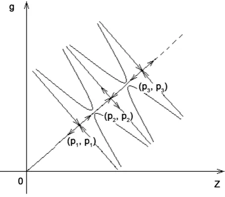
6. Physical Dynamic Boundary Conditions

Let us consider the following model [2]: δn I

( )

=klnI I_t, where δn I

( )

is refractive

(13)

Figure 2. Phase portrait for simplest solutions of relaxation type (white and black solitons).

(

p p1, 1

) (

, p p3, 3

)

-attractive

fixed points,

(

p p2, 2

)

-saddle point of co-dimensional 1.

study propagation of a spatially incoherent, quasi-monochromatic and linearly po- larized light beam in a linear photopic lattice with a non-instantaneous surface nonlinearity. The electron field fluctuates on time scale much shorter than the response time of the nonlinearity [4]. The state of the system can be described by a function

( )

_, *

( ) ( )

_, _, _,

I x t = E x t E x t , where E is the electric field, E* is the value which is

conjugate to the value E.

Now we show how can be postulated nonlinear boundary conditions. For plane waves the density is defined as

2

0 0

1

2 l

I= c n Eε (79)

where c is velocity of light, nl is linear refractive index at low fields. The effective

refractive index can be written as

( ) ( )

1 2 2 1

2 0

3

1 .

2 2

eff

l

n I

c n

χ χ

ε

 

=_ + + _

  (80)

Indeed, as noted in [10]: “the nonlinear effects in optical fiber occur either due to intensity dependence of refractive index of the medium or due to inelastic-scattering phenomenon”. There are various types of nonlinear effects based on self-phase modulation, cross-phase modulations and four-wave mixing. We consider the effect when the refractive index is the nonlinear function of the optical intensity. The power dependence describes the Kerr-effect [10]. Origin of nonlinearity is the unharmonic motion of electrons under the action of the polarization , which is induced by electric dipoles so that

( )1 ( )2 2

0 E 0 E

ε χ ε χ

= + +

[image:13.595.260.488.72.271.2]

(14)

where ε0 is the permittivity of vacuum and

( )

, 1, 2,

k

χ = __{is susceptibility.}

We assume that there is the surface polarization at a walls which confine the laser fiber. Then defects and color centers at the walls produce the second order gene- ralization. We confined itself by the study only the quadratic boundary conditions which describes wave type distributions of relaxation, pre-turbulent and turbulent type. Then the surface refractive index is δn=neff

( )

I I . Then one of the boundary con-

ditions can be written as

( )

_0, 1

( )

_0, _,

( )

_, 2

( )

_, _.

eff eff

I I

t n I t l t n I l t

x t

∂ ₌ ∂ ₌

∂ ∂ (82)

In similar form, we can consider more common boundary conditions. Then from (80) it follows that ( )1 ( )2

,

χ χ _{are bifurcations parameters. Formally, their changing leads to}

appearing of period doubling distributions bifurcations and, correspondingly, to ex- istence of distributions of relaxation, pre-turbulent and turbulent type. We can consider also the values ( )1

1 1

µ = +χ _and ₂ ( )2 ₂ 0 3 2 2c n_l

χ µ

ε

= as bifurcations parameters.

From the formula δn I

( )

=klnI I_t it follows that we can use the approximation

(

)

1

(

)

2 1

(

)

3 ln 1

2 3

t t t t

I I I I I I I I

+ = − + +_₍₈₃₎

for I It1 unless I It= −1. Then the boundary conditions can be written as

( )

1

( )

2

( )

0, eff 0, , , eff ,

I I

t n I t l t n I l t

x t

∂ ₌ ∂ ₌

∂ ∂ (84)

if neffk =nlk+I I kt, =1, 2. Thus we obtain the problem with nonlinear boundary

conditions which can be considered as above. Here, k l

n is a bifurcation parameter.

7. Applications to Semiconductor Lasers

In semiconductor lasers, the intersection field matter is realized through the carrier density n which satisfies to the equation [3]:

2 2

2

s a

n j n g n

E D

t qv τ ω x

∂ ₌ ₋ ₋ ₊ ∂

∂  ∂ (85)

where I ~ E , j is the injection current, q is the electron charge, v is active volume of

the device, τs is lifetime of the carriers, g is optical gain in cm−1, and D is the diffusion

coefficient.

We assume that device is placed at a point x=0, and the Neumann boundary

condition

0 at 0.

n

x x

∂ ₌ ₌

∂ (86)

Next, we assume that the media of semiconductor laser is ideal that is light propagates throw the media without changing of amplitude along lines d dx t=V ,

(15)

1

at 0.

s a

j

n n g

x

t qv τ ω

∂ ₌ ₋ ₋ ₌

∂  (87)

We assume that

(

)

2

a

g=a n−n −E (88)

where na is the carrier density at transparency,  is the gain compress factor. As

noted in [3]: “the actual dependence of the gain on the field density is still object of controversy”. Note that in the paper [3] has been considered the case 2

1 E ll

 .

Next, we consider, additionally, the boundary conditions

2

at

s

j

n n

x l

t qv τ

∂ ₌ ₋ ₌

∂ (89)

that is 2 1

I  at x=0.

On the other hand, from the theory of the injection locking it follows that

(

)

(

)

(

2

)

1 1

1

1 at 0

2 a

I

a n n I x

t γ

∂ _{= −} ₋ ₋ ₋ ₌

∂ (90)

where γ1,a n1, a are constants. Assuming that 2

1

I  at x=l, we obtain the right

boundary condition

(

)

(

1 1

)

1

at .

2 a

I

a n n x l

t γ

∂ _{= −} ₋ ₋ ₌

∂ (91)

Thus we get the dynamic boundary conditions. Applying the method of reduction corresponding initial value boundary problem to a system of difference equations, we obtain that the problem has solutions of relaxation, pre-turbulent and turbulent type for a special case of the coefficients γ1,a n1, a and so on.

8. Comparison with Experiment

In [9] has beeb discusses the dynamics of modulation surface directed instability and periodic waves in the coupled linear equations which describes light propagation in dispersed Kerr media. New spatial-temporal periodic solutions are found for these equations. As noted in [9]: there is “the fundamental link which exists between the phenomenon of polarization instability and the so-called black and white vector solitons”. From this point of view, the asymptotic periodic spatial-temporal periodic solutions obtained in our paper are not the solitons, because solitons exists due to a balance between surface induced injection of radiation into optic media and volume radiation. Surface radiation with feedback can be modeled by laser diode. The balance can be achived only asymptotically as t→ ∞. We obtain white and black asymptotic

impulse the form of which determined by the form of surface induced impulse. In this case, parameters of surface absorption and emission are bifurcation parameter which define the period and the frequency oscillations on the period white and black “solitons” [11].

Spatial solitons were experimentally observed in 1997 by Mitchel and Segev (see,

(16)

dynamic balance between the tendency for the beam to expend as a result of diffraction and the property of beam to contract as a result of self focusing. In [23] has been demonstrated solitons which can be obtained from both the spatially and temporally incoherent light. But, as noted in [11], the corresponding theory can not explain spatial-temporal coherence properties and also properties of temporal spectral density of such solitons. We believe that the initial value boundary problem, which is considered in the present paper, may be useful to describe formal properties of spatial- temporal solitons and their spectral properties.

9. Conclusion

In this paper, we analyze the dynamic of surface, and induce nonlinear instability in ideal optic volume producing light propagation, reflected from walls, which confines an ideal resonator. The problem is described by two linear difference equations with nonlinear dynamic boundary conditions for density of radiations and density of photons in the resonator. It is shown that deriving from the form of the boundary conditions with feedback we can obtain distributions of the light of relaxation, pre- turbulent and turbulent type.

References

[1] Faccio, D. (2012) Laser Pulse Analogues for Gravity and Analogues Hawking Radiation.

Contemporary Physics, 93, 97-112.http://dx.doi.org/10.1080/00107514.2011.642559

[2] Jablan, M., Buljan, H., Manela, O. and Segev, M. (2007) Incoherent Modulation Instability in a Nonlinear Photonic Lattice. Optics Express, 15, 4623-4633.

http://dx.doi.org/10.1364/OE.15.004623

[3] Mecozzi, A., D’Ottavi, A. and Hui, R. (1993) Nearly Degenerated Four-Wave Mixing in Disturbed Feedback Semiconductor Lasers Operating above Threshold. Journal of

Quan-tum Electronics, 29, 1477-1487.http://dx.doi.org/10.1109/3.234398

[4] Sljačić, M., Segev, M., Coskuna, T.H., et al. (2000) Modulation Instability of Incoherent Beams in Non-Instantaneous Nonlinear Media. Physical Review Letters, 84, 467-470. http://dx.doi.org/10.1103/PhysRevLett.84.467

[5] Demircan, A., Amiranashvili, Sh. and Steinmeyer, G. (2011) Controlling Light by Light with an Optical Event Horizon. Physical Review Letters, 106, 163901-163907.

http://dx.doi.org/10.1103/PhysRevLett.106.163901

[6] Webb, K.E., Erkintalo, M., Broderick, N.G.R., Dudley, J.M., Broderick, N.G.R., et al. (2014) Nonlinear Optics of Event Horizons. Nature Communications, 5, Article Number: 4969. [7] Coven, E.M. and Hedlung, G.A. (1980) Continuous Maps on the Interval Whose Periodic

Points Form a Closed Set.Proceedings of the American Mathematical Society, 79, 127-133. http://dx.doi.org/10.1090/S0002-9939-1980-0560598-7

[8] Philbin, T.G., et al. (2008) Fiber-Optical Analog of the Event Horizon. Science, 319, 1367- 1370.http://dx.doi.org/10.1126/science.1153625

[9] Haelterman, M. (1994) Modulational Instability, Periodic Waves and Black and White Vector Solitons Birefringent Kerr Media. Optics Communications, 11, 86-92.

http://dx.doi.org/10.1016/0030-4018(94)90144-9

(17)

and Applications. Progress in Electromagnetic Research, 73, 249-275. http://dx.doi.org/10.2528/PIER07040201

[11] Buljan, H. and Segev, M. (2003) White-Light Solitons. Optics Letters, 28, 1239-1241. http://dx.doi.org/10.1364/OL.28.001239

[12] Sharkovsky, A.N., Maistrenko, Yu.L. and Romanenko, E.Yu. (1993) Difference Equations and Their Applications. Ser. Mathimatics and Its Applications. Kluwer Academic, Dor-drecht.

[13] Galenko, P. and Jou, D. (2005) Diffuse-Interface Model for Rapid Phase Transformations in with Relaxation of the Diffusion Flux in Nonequilibrium Systems. Physical Review E, 71, Article ID: 046125.http://dx.doi.org/10.1103/PhysRevE.71.046125

[14] Lecoq, N., Zapolsky, H. and Galenko, P. (2009) Evolution of the Structural Factor in a Hyperbolic Model of Spinodal Decomposition. Physical Review E, 177, 165-175.

[15] Galenko, P. and Jou, D. (2009) Kinetic Contribution to the Fast Spinodal Decomposition Controlled by Diffusion. Physica A: Statistical Mechanics and Its Applications, 388, 3113- 3123.http://dx.doi.org/10.1016/j.physa.2009.04.003

[16] Lecoq, N., Zapolsky, H. and Galenko, P. (2009) Evolution of the Structure Factor in a Hyperbolic Model of Spinodal Decomposition. European Physical Journal Special Topics, 179, 165-175.http://dx.doi.org/10.1140/epjst/e2009-01173-8

[17] Krasnyuk, I.B., Taranets, R.M. and Yurchenko, V.M. (2010) Pulse Structures Lamellar Type in the Bounded Polymeric Systems. Matematicheskoe Modelirovanie, 22, 65-81.

[18] Krasnyuk, I.B. and Taranets, R.M. (2009) The Spatiotemporal Oscillations of Order Para-meter for Isothermal Model of the Surface-Directed Spinodal Decomposition in Bounded Binary Mixtures. Research Letters in Physics, 2009, Article ID: 250203.

http://dx.doi.org/10.1155/2009/250203

[19] Krasnyuk, I.B. and Taranets, R.M. (2011) The Spatial-Temporal Lamellar Structures in the Confined Ideal Polymer Blends. Journal of Statistical Physics, 145, 1485-1498.

http://dx.doi.org/10.1007/s10955-011-0378-5

[20] Brandenburg, A., Käpylä P.J. and Mohammed, A. (2004) Non-Fickian Diffusion and Tau Approximation for Numerical Turbulence. Physic of Fluids, 16, 1020-1028.

http://dx.doi.org/10.1063/1.1651480

[21] Maxwell, J.C. (1867) On the Dynamical Theory of Gases. Philosophical Transactions of the

Royal Society, 157, 49-88.http://dx.doi.org/10.1098/rstl.1867.0004

[22] Libenson, M.N., Jakovlev, E.B. and Shandibina, R.I. (2008) The Interaction of Radiation with Matter C Substance (Optical Power). ITMO, St. Petersburg.

[23] Mitchell, M., Chen, Z., Shih, M. and Segev, M. (1996) Self-Trapping of Partially Spatially Incoherent Light. Physical Review Letters, 77, 490-495.

(18)

Submit or recommend next manuscript to SCIRP and we will provide best service for you:

Accepting pre-submission inquiries through Email, Facebook, LinkedIn, Twitter, etc. A wide selection of journals (inclusive of 9 subjects, more than 200 journals)

Providing 24-hour high-quality service User-friendly online submission system Fair and swift peer-review system

Efficient typesetting and proofreading procedure

Display of the result of downloads and visits, as well as the number of cited articles Maximum dissemination of your research work

Submit your manuscript at: http://papersubmission.scirp.org/