http://www.scirp.org/journal/tel ISSN Online: 2162-2086 ISSN Print: 2162-2078
DOI: 10.4236/tel.2016.66115 November 21, 2016
Rationalizing Irrational Beliefs
Geoffrey Dunbar
1,2, Ruqu Wang
3, Xiaoting Wang
4*1International Economic Analysis Department, Bank of Canada, Ottawa, Canada 2Department of Economics, University of Ottawa, Ottawa, Canada
3Economics Department, Queen’s University, Kingston, Canada 4Department of Economics, Acadia University, Wolfville, Canada
Abstract
In this paper we propose a “behavioral equilibrium” definition for a class of dynamic games of perfect information. We document various experimental studies of the Centipede Game in the literature that demonstrate that players rarely follow the subgame perfect equilibrium strategies. Although some theoretical modifications have been proposed to explain the outcomes of the experiments, we offer another: players can choose whether or not to believe that their opponents use subgame per-fect equilibrium strategies. We define a “behavioral equilibrium” for this game; using this equilibrium concept, we can reproduce the outcomes of those experiments.
Keywords
Centipede Game, Game Theory, Experimental Economics, Behavioral Economics
1. Introduction
In dynamic games of perfect information, the concept of subgame perfect equilibrium is most commonly used in the prediction of players’ behavior. Consider a generic game of finitely many moves, the subgame perfect equilibrium always uniquely exists. While the equilibrium concept is easily understood and the equilibrium characterization is usually straightforward, challenges to its ability to predict players’ behavior grow in the literature, both on theoretical front and experimental front.
Rosenthal [1] constructed a game (later dubbed the “Centipede Game”) that consisted of a sequence of one hundred moves. In this game, each player moves in every alternative period, either to pass (to the next period) or to end the game right away. Passing the game to the next period yields a larger total pile of money, but it strictly reduces the payoff a player receives if the opponent ends the game in her subsequent turn. The unique sub-*Corresponding author.
How to cite this paper: Dunbar, G., Wang, R.Q. and Wang, X.T. (2016) Rationalizing Irrational Beliefs. Theoretical Economics Letters, 6, 1219-1229.
http://dx.doi.org/10.4236/tel.2016.66115
Received: October 10, 2016 Accepted: November 18, 2016 Published: November 21, 2016 Copyright © 2016 by authors and Scientific Research Publishing Inc. This work is licensed under the Creative Commons Attribution International License (CC BY 4.0).
1220
game perfect equilibrium (SPE) is that the first player ends the game at the first node and each player gets a small sum. Rosenthal argued that it is highly unlikely that, in practice, players will actually choose the SPE strategies when they play that game.
Various centipede game experiments have been conducted to test the predictive power of the concept of SPE. McKelvey and Palfrey [2] reported that only 15% of the players end the game at the first node (the outcome predicted by SPE) in a high-payoff version, and that number reduces to as little as 0.7% in other versions of the centipede game. In a much simplified two-move extensive form game, Goeree and Holt [3] do-cumented that players usually did not trust their opponents to be rational. In contrast, Palacios-Huerta and Volij [4] conduct experiments involving expert chess players, who are known for their high degree of rationality and ability to find optimal strategies us-ing backward induction reasonus-ing. The outcome of their experiments is very close to the SPE prediction. Overall these experimental studies suggest that common knowledge of rationality of all players is the key requirement of SPE and so it is not surprising that players do not follow SPE strategies if they do not believe their opponents are rational.
In an attempt to reconcile the differences between the theory and the experimental outcomes, various modifications to the assumptions of the games used in the experi-ments have been proposed. McKelvey and Palfrey [2], for example, propose that a player believes that the opponent is an altruist with some positive probability. They find that even a very small such probability can induce players to adopt mixed strategies in the early rounds of the game, mimicking the observed behaviors in their experiment1. A few years later, McKelvey and Palfrey [6] use a quantal choice model to re-examine the same experimental results. They show that if one assumes that the probability of im-plementing a particular strategy is increasing in the equilibrium payoff of the strategy, then the observed behavior more or less coincides with the predictive behavior. Zauner [7] proposes an alternative explanation of McKelvey and Palfrey’s experimental results by assuming a random perturbation of each player’s payoffs. He considers different types of perturbations and two best-fit models are selected.
In the theoretical literature, game theorists have proposed alternatives to some key assumptions that lead to SPE, including the common knowledge of rationality and backward induction. Aumann [8] formalizes the idea of higher order mutual know-ledge2. Caplan [10] treats irrationality as a standard good, and players need to pay to get closer to some (irrational) “bliss belief.” Basu [11] argues that each history of moves reveals certain characteristics of players to one another, and therefore the outcomes of a game depend on these revealed characteristics (instead of depending on rationality alone). Halpern and Pass [12] propose the “iterated regret minimization” as a solution concept for strategic games. They apply it to the centipede games and find that, with li-near payoffs, players will cooperate for a number of rounds. With exponential payoffs, they will cooperate all the way up to the end of the game. Meanwhile, Rand and Nowak
1In an indirect evolutionary model in which a centipede game is played in each stage, Gamba [5] shows that
altruism can evolve even if preferences are unobservable.
2Samet [9] labels the material rationality in a centipede game as common belief instead of common
1221
[13] model the stochastic evolution of strategies in the centipede game and find that the players’ cooperative behavior may in fact be the favored outcome of natural selection.
Advances in psychology also help explain why players in experiments may behave differently than SPE predicts. Epstein et al. [14] conduct studies that test the cogni-tive-experiential self-theory. They confirm that two conceptual systems, an experiential system and a rational system, operate by their own rules of inference inside the same individual. To some extent, an individual may switch from one system to another. Ti-role [15] builds on similar psychological findings and proposes a model of rational irra-tionality that can explain why people rehearse good news and selectively forget bad news—a universal behavior.
In this paper, we argue along the lines of the above psychological findings and pro-pose another theoretical explanation of the failure of the SPE as a predictor of behavior. We emphasize on the observation that even if all players understand fully the concept of subgame perfect equilibrium and even if no players believe that other players are al-truists, they still do not follow the SPE strategies when playing the centipede game. We assume that a player can choose to play SPE, i.e. be “rational”, or else may choose to be “behavioral”. If being “behavioral” yields a better expected outcome than being “ration-al”, then a player would choose to be “behavioral” (or, in terms of standard game theory terminology, “irrational”). Our intuition is as follows. SPE strategies are optimal for a player only when other players follow them. If players do not believe that other players will follow SPE strategies, then their own SPE strategies are not, in general, op-timal. In the model, we specify an alternative belief for each player regarding the beha-vior of other players. Each player then has a choice of selecting his belief (between the SPE strategy and the alternative one) at the beginning of the game and then optimizing given the selected belief. A “behavioral equilibrium” is formed if each player is better off in the actual outcomes by selecting the alternative belief. These outcomes of the game are determined by the strategies the players actually used in the game.
The basic idea behind the “behavioral equilibrium” concept is that players can choose to believe that their counterparts can be either fully rational (such that SPE strategies are the best response) or somewhat irrational (so that SPE strategies are not best response any more). Given any belief, the players still optimize by choosing the best strategy. This is the same as in a subgame perfect equilibrium. However, the dif-ference between a behavioral equilibrium and a subgame perfect equilibrium is that those alternative beliefs in a behavioral equilibrium do not usually coincide with those players’ actual strategies. If the two are the same, a subgame perfect equilibrium is formed. Therefore, these alternative beliefs are somewhat irrational. Still, these irra-tional beliefs generate better payoffs than those SPE beliefs. Thus, players will choose these irrational beliefs rationally.
ra-1222
tional system. As we observed in the above-mentioned experiments, players are better off using the irrational beliefs than the rational beliefs. These irrational beliefs may not translate into the players’ “maximum” payoffs. But the payoffs are usually very good, and are much better than the payoffs implied by SPE strategies. Therefore, players may reinforce these irrational beliefs and move away from their rational beliefs. In some sense, these irrational beliefs are the “rules of thumb” for the players.
One real life example related to the centipede games that we examine in this paper is the rotating-savings and credit associations (Roscas), commonly found in many devel-oping countries. (See Besley et al. [16] and Anderson and Baland [17], for example.) In these associations, a predetermined group of individuals get together and contribute a predetermined amount into a “pool” which is then given to one member (winner). These gatherings repeat themselves, with previous winners excluded from receiving the “pool” while still being obliged to contribute. The gathering may stop after each mem-ber has received the “pool” but often the same group continues the Rosca with a new “pool”. These Roscas run the risk of earlier winners defaulting on later contributions, a strategy resembling “stopping early” in the centipede game. Still, defaults are very in-frequent. Our model of “irrational beliefs” or “rules of thumbs” may shed some light on these phenomena.
The rest of this paper is organized as follows. In Section 2, we analyze a few centipede games using the concept of “behavioral equilibria”. In Section 3, we analyze some of the experiments in centipede games in the literature. In Section 4, we conclude.
2. Centipede Games and Behavioral Equilibria
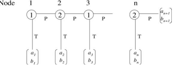
We begin with a general description of the centipede games.There are two players, 1 and 2, playing the centipede game of n moves in Figure 1. To simplify notation, we assume that n is even.
In this game, a1>a2 , a3 >a4,
, a2i−1>a2i, , an−1 >an , and b2 >b3, 4 5b >b ,
, b2j−2 >b2j−1, , bn>bn+1. It is straight-forward to check that theunique subgame perfect equilibrium strategy for each player is to play T whenever it is his turn to move. Given this strategy, the equilibrium outcome of the game is that play-er 1 plays T at the very beginning and ends the game with payoffs
(
a b1, 1)
. [image:4.595.231.524.579.689.2]Now suppose that before the start of the game, the two players choose a belief secret-ly and simultaneoussecret-ly. Player 1 chooses a belief from
{
SPE B1, 1}
; at the same time,1223 player 2 chooses a belief from
{
SPE B2, 2}
. Here, SPEi represents player i’s subgame perfect equilibrium belief on his opponent j’s behavior; i.e., player j will play T whenev-er it is his move. On the othwhenev-er hand, Bi denotes player i’s alternative belief. Let(
)
1 2, 4, , n
B = p p p be player 1’s belief, where p2k is the probability that player 2
will play T at node 2k conditional on node 2k being reached. For SPE belief,
(
)
1 1,1, ,1
SPE = . Similarly, we define B2 =
(
p p1, 3,,pn−1)
, and SPE2=(
1,1,,1)
.The subgame perfect equilibrium belief SPEi is the only belief that satisfies the properties of common knowledge of rationality and backward induction in the centi-pede game. Therefore, any other belief Bi would violate at least one of these proper-ties. This alternative belief may be derived from a player’s past game-play experience against other players and/or some “rules of thumb” guesses may have been formed. Since players in general do not always behave rationally, these “rules of thumb” guesses do not always coincide with the other players’ SPE strategies.
In summary, the game we are examining is as follows. Both players simultaneously select their beliefs before the start of the game. Once the belief is selected, it remains the same throughout the game. Given these beliefs regarding an opponent’s behavior, play-ers play the above centipede game. Each player’s goal is to maximize his expected payoff given his chosen belief.
To simplify our analysis, we assume that the beliefs are not updated during the game. (Even if we allow for belief updating, we will not get back the SPE beliefs as long as the initial belief is somewhat incorrect.)
To analyze the modified centipede game, first note the following. If B1 is such that
playing T at node 1 is the optimal action for player 1, then the game is over at node 1 no matter what belief player 1 has selected. The more interesting case is when playing T
at node 1 is not the optimal action.
If player 1 chooses belief SPE1 and thus plays T at the first node, the game ends at
the first node, with payoffs
(
a b1, 1)
. If player 1 chooses belief B1, player 1 maximizeshis expected payoff by choosing the node he plans to play T:
{ }
(
)
(
)(
) (
)
(
)(
) (
)(
)
2 2 2 4 5 2 4 3 1 1 1,3, , 1
2 4 3 1
max 1 1 1 1
1 1 1 1
i i i
i n
i i i
p a p p a p p p p a
p p p p a
− − − ∈ − − − + − + + − − − + − − − − (1)
Let * 1
i=n denote an i that maximizes the above. (Note that there could be many
such i’s that maximize the above.) Consider player 2 at node 2. The optimal action with the belief of SPE2 is to end the game right away. In this case, the payoffs are
(
a b2, 2)
. If belief B2 is chosen, player 2 maximizes his expected payoff by choosing the node heplans to play T:
{ }
(
)
(
)(
)
(
)
(
)(
)
(
)(
)
1 1 1 3 3 1 3 3 1 1
2,4, ,
1 3 3 1
max 1 1 1 1
1 1 1 1
j j j
j n
j j j
p b p p b p p p p b
p p p p b
− − − ∈ − − + − + + − − − + − − − − (2)
Let * 2
j=n denote a j that maximizes the above. (Again, there could be many such
j’s that maximize the above.)
1224
* 1
n . The proposed pure strategy for player 2 is to select B2 and play P at node 2 (if
player 1 played P at node 1), and plan to play T at node * 2
n . The game ends at node
{
* *}
*1 2
min n n, ≡n .
Definition 1
{
B n1, 1}
∗ and
{
}
2, 2
B n∗ form a pure strategy “behavioral equilibrium”
if player 1’s payoff is higher by selecting
{
B n1, 1}
∗ than selecting
{
}
1,1SPE given
player 2’s strategy of playing T at node n2
∗, and player 2’s payoff is higher by selecting
{
B n2, 2}
∗ than selecting
{
}
2,1SPE given player 1’s strategy of playing T at node n1∗.
That is,
1, and 2,
n n
a∗ ≥a b∗≥b
where n min
{
n n1, 2}
∗ = ∗ ∗ .
In this behavioral equilibrium, players are better off selecting these non-SPE beliefs than selecting the SPE beliefs. These beliefs are reinforced if the players play these games again later.
Now consider mixed strategy “behavioral equilibria”. Suppose that there are more than one j’s that maximize (2), or there are more than one i’s that maximize (1), mixed strategies could be used by the players. Let
(
)
1 2
1 , , , , , ,
k
i i i
s = q∗ q∗ q∗ denote any of
player 1’s optimal mixed strategies, where i i1, ,2 ,ik
∗ ∗ ∗ are all of the numbers that maximizes (1). Similarly, let
(
)
1 2
2 , , , , , ,
k
j j j
s = q∗ q∗ q∗ denote any of player 2’s
optimal mixed strategies, where j1,j2, ,jk
∗ ∗ ∗ are all of the numbers that maximizes (2). Then the outcomes of the game are determined by s1 and s2.
Definition 2
{
B s1, 1}
∗ and
{
}
2, 2
B s∗ form a mixed-strategy “behavioral
equili-brium” if player 1’s payoff is higher by selecting
{
B s1, 1}
∗ (comparing to
{
}
1,1SPE )
given player 2’s strategy s2
∗, and player 2’s payoff is higher by selecting
{
}
2, 2
B s∗
(comparing to
{
SPE2, 2}
) given player 1’s strategy s1 ∗.Again, in this behavioral equilibrium, players are better off selecting these non-SPE beliefs than selecting those SPE beliefs. We can generalize the concept of behavioral equilibria to any general game G with n players and normal-form payoff
(
1, 2, ,)
i
n
s s s
Π , i=1, 2,, .n
Definition 3 Suppose that σ =
(
σ σ1, 2,,σn)
is a subgame perfect equilibriumstrategy profile in G. Let SPEi =σ−i =
(
σ1,,σi−1,σi+1,,σn)
be player i’s subgameperfect equilibrium belief about other players’ strategies. Suppose that
(
1, , 1, 1, ,)
i i i i
i i i n
B = s s− s+ s be player i’s another belief about other players’ strategies
and si
∗ is player i’s best response to i
B . Then
{
}
1, ,
, i i
i n
B s∗
= form a “behavioral
equi-librium” if
(
1, 2, ,)
(
1, 2, ,)
i i
n n
s s∗ ∗ s∗ σ σ σ
Π ≥ Π , i=1, 2,, .n
Note that in the above definition, a player’s belief may not be correct; that is, Bi is not necessarily the same as s i
(
s1, ,si1,si1, ,sn)
∗ ∗ ∗ ∗ ∗
− = − + . However, the optimal res-ponses to these “incorrect” beliefs generate higher payoffs to each player than the sub-game perfect equilibrium payoffs. Therefore, these “incorrect” beliefs are reinforced.
Note also that the subgame perfect equilibrium strategy profile σ together with the
1225 using the dominant strategies are the unique behavioral equilibrium, since they are op-timal independent of players’ beliefs.
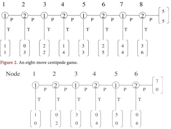
Below, we focus on centipede games to illustrate our equilibrium concept. Example 1 Consider the eight-move centipede game in Figure 2.
Suppose that B1=
(
0, 0, 0,1)
and B2=(
0, 0, 0,1)
. Then it is straight-forward to ob-tain n1 7∗= , and
2 6
n∗= . That is, player 1 playing T at node 7 is optimal given B1,
while player 2 playing T at node 6 is optimal given B2. The minimum of n1 ∗ and
2
n∗, n∗, is 6; that is, the game ends at node 6, with payoffs (2,5).
It is easy to see that
{
*}
1, 1B n and
{
B n2, *2}
form a behavioral equilibrium because* 1
n
a >a , and bn* >b2.
Example 2 Consider the six-move centipede game in Figure 3.
In this game, we can construct pure-strategy behavioral equilibria similarly to the last example. Let B1=
(
0,1, 0)
, and B2 =(
0, 0,1)
. Then we have n1 3∗ = , and
2 4
n∗= .
Therefore, n min
{
n n1, 2}
3∗= ∗ ∗ = ; that is, the game ends at node 3. This constitutes a behavioral equilibrium as the final outcome is (3,0), which is weakly better for both players than the SPE outcome of (1,0).
Now consider a mixed-strategy behavioral equilibrium. Suppose that B1=
(
0,p4,1)
and B2=(
0,p3,1)
, with p4∈( )
0,1 and p3∈( )
0,1 . Given these beliefs, denote play-er 1’s expected payoff of planning to play T at node i by EΠ1( )
i . We have( )
1 1 1
EΠ = , EΠ1
( )
3 =3, and EΠ1( )
5 = p40+ −(
1 p4)
5. For player 1 to randomizebetween playing T at node 3 and playing T at node 5, we should set EΠ1
( )
3 = ΠE 1( )
5 ; that is, 42 5
p = .
[image:7.595.206.546.436.691.2]Similarly, for player 2, EΠ2
( )
2 =2, EΠ2( )
4 =p30+ −(
1 p3)
4, and EΠ2( )
6 =0.Figure 2. An eight-move centipede game.
1226
Suppose that 3
1 2
p < . Then *
2 4
n = .
To construct a behavioral equilibrium, player 1’s mixed strategy
(
0,q3,1)
must sa-tisfy the following two conditions regarding each player’s actual payoffs. First, for play-er 1, q33+ −(
1 q3)
0 is at least 1, which is player 1’s payoff by following SPE strategy and playing T at node 1. This gives us 31 3
q ≥ . Second, for player 2, q30+ −
(
1 q3)
4 must be at least 2, which is player 2’s payoff by following SPE strategy and playing T at node 2. This gives us 31 2
q ≤ . Therefore, any 3
1 1 , 3 2
q ∈
would satisfy these two
conditions.
To summarize, 1
2 0, ,1
5
B =
, s1 =
(
0,q3,1)
, B2=(
0,p3,1)
, s2=(
0,1,1)
, where3
1 1 , 3 2
q ∈
, and 3
1 0,
2
p ∈
form a mixed-strategy behavioral equilibrium.
3. Analyzing Previous Centipede Game Experiments
McKelvey and Palfrey [2] report the results of seven different centipede game experi-ments. Sessions 1 to 3 are four-move centipede games with the following payoffs:
(
a b1, 1) (
= 0.4, 0.1)
,(
a b2, 2) (
= 0.2, 0.8)
,(
a b3, 3) (
= 1.6, 0.4)
,(
a b4, 4) (
= 0.8, 3.2)
, and(
a b5, 5) (
= 6.4,1.6)
.3 Session 4 is a high-payoff four-move centipede game where the payoffs are quadrupled. Sessions 5 to 7 are six-move centipede games with the follow-ing payoffs:
(
a b1, 1) (
= 0.4, 0.1)
,(
a b2, 2) (
= 0.2, 0.8)
,(
a b3, 3) (
= 1.6, 0.4)
,(
a b4, 4) (
= 0.8, 3.2)
,(
a b5, 5) (
= 6.4,1.6)
,(
a b6, 6) (
= 3.2,12.8)
, and [image:8.595.190.554.94.295.2](
a b7, 7) (
= 25.6, 6.4)
.Table IIA in McKelvey and Palfrey [2] reports the proportion of observations at each terminal node. In that table, fi is used to denote the proportion of games that ends at node i. From these fi’s, we can calculate a player’s strategy as follows. For the four-move game, let q1 and q3 be the proportion of player 1 who plans to choose
TAKE at node 1 and at node 3 respectively. (Therefore, the proportion of player 1 choosing Pass at node 3 is equal to 1− −q1 q3.) Similarly, let q2 and q4 be the
pro-portion of player 2 who plan to choose TAKE at node 2 and at node 4 respectively, and thus the proportion of player 2 choosing Pass at node 4 is equal to 1−q2−q4. Then
1 1
q = f ,
(
1−q q1)
2= f2,(
1−q2)
q3= f3, and(
1− −q1 q q3)
4 = f4. We define qi si-milarly in the six-move game. Then we have q1= f1,(
1−q q1)
2 = f2,(
1−q2)
q3= f3,(
1− −q1 q q3)
4 = f4,(
1−q2−q4)
q5= f5, and(
1− −q1 q3−q5)
q6 = f6. The results are reported in the following table.We cannot infer a player’s belief in playing these games from the data since many different beliefs could lead to the same observed strategy. Therefore, in each session, we assume that a player’s belief corresponds exactly to his rival’s revealed strategy and cal-culate the player’s optimal action according to that belief. In the calculations, we assign the players a utility function with a constant degree of absolute risk aversion of 0.5 so
3Payoffs
(
) (
)
5, 5 6.4,1.6
1227
Table 1. Players’ strategies and optimal actions.
Session q1 q2 q3 q4 q5 q6 Optimal Action
1 player 1 0.06 0.61 Take at Node 3 (61%)
player 2 0.28 0.61 Take at Node 4 (61%)
2 player 1 0.10 0.69 Take at Node 3 (69%)
player 2 0.42 0.52 Take at Node 4 (52%)
3 player 1 0.06 0.42 Pass at Node 3 (42%)
player 2 0.46 0.33 Take at Node 4 (33%)
4 player 1 0.15 0.57 Take at Node 3 (57%)
player 2 0.44 0.39 Take at Node 2 (44%)
5 player 1 0.02 0.43 0.50 Take at Node 5 (50%)
player 2 0.09 0.51 0.20 Take at Node 4 (51%)
6 player 1 0.00 0.04 0.70 Take at Node 5 (70%)
player 2 0.02 0.48 0.42 Take at Node 4 (48%)
7 player 1 0.00 0.15 0.55 Take at Node 5 (55%)
player 2 0.07 0.51 0.40 Take at Node 4 (51%)
that the players are modestly risk averse. That is,
( )
0.5e x
i
U x = − − for player i, where
x is the amount of money earned in one game. The results are reported in Table 1 as well. The percentage number after each optimal action is the percentage of players actually choosing the implied optimal action in that session. As we can see from the table, the majority of the players chose the implied optimal action in all but session 3. We interpret these findings cautiously as our assumption that a player’s belief cor-responds exactly to his rival’s revealed strategy is only one possible specification of beliefs consistent with the behavioral equilibrium. Nevertheless, and in contrast with the predictions of SPE, the behavior of the majority of the players can be explained by our theory.
4. Conclusion
1228
Acknowledgements
We thank the referees, Jim Bergin, Lester Kwong and Jasmina Arifovic for helpful com- ments. Ruqu Wang’s research is supported by the Social Sciences and Humanities Re-search Council of Canada. Xiaoting Wang acknowledges support from the National Natural Science Foundation of China (#71571038).
References
[1] Rosenthal, R. (1982) Games of Perfect Information, Predatory Pricing, and the Chain Store Paradox. Journal of Economic Theory, 25, 92-100.
https:/doi.org/10.1016/0022-0531(81)90018-1
[2] McKelvey, R. and Palfrey, T. (1992) An Experimental Study of the Centipede Game. Eco-nometrica, 60, 803-836. https:/doi.org/10.2307/2951567
[3] Goeree, J. and Holt, C. (2001) Ten Little Treasures of Game Theory and Ten Intuitive Con-tradictions. American Economic Review, 91, 1402-1422.
https:/doi.org/10.1257/aer.91.5.1402
[4] Palacios-Huerta, I. and Volij, O. (2009) Field Centipedes. American Economic Review, 99, 1619-1635. https:/doi.org/10.1257/aer.99.4.1619
[5] Gamba, A. (2013) Learning and Evolution of Altruistic Preferences in the Centipede Game.
Journal of Economic Behavior & Organization, 85, 112-117. https:/doi.org/10.1016/j.jebo.2012.11.009
[6] McKelvey, R. and Palfrey, T. (1998) Quantal Response Equilibria for Extensive Form Games. Experimental Economics, 1, 9-41. https:/doi.org/10.1023/A:1009905800005
[7] Zauner, K. (1999) A Payoff Uncertainty Explanation of Results in Experimental Centipede Games. Games and Economic Behavior, 26, 157-185.
https:/doi.org/10.1006/game.1998.0649
[8] Aumann, R. (1992) Irrationality in Game Theory. In: Dasgupta, P., et al., Eds., Economic Analysis of Markets and Games: Essays in Honor of Frank Hahn, MIT Press, Cambridge and London, 214-227.
[9] Samet, D. (2013) Common Belief of Rationality in Games of Perfect Information. Games and Economic Behavior, 79, 192-200. https:/doi.org/10.1016/j.geb.2013.01.008
[10] Caplan, B. (2001) Rational Irrationality and the Microfoundations of Political Failure. Pub-lic Choice, 107, 311-331. https:/doi.org/10.1023/A:1010311704540
[11] Basu, K. (1988) Strategic Irrationality in Extensive Games. Mathematical Social Sciences, 15, 247-260. https:/doi.org/10.1016/0165-4896(88)90010-8
[12] Halpern, J. and Pass, R. (2012) Iterated Regret Minimization: A New Solution Concept.
Games and Economic Behavior, 74, 184-207. https:/doi.org/10.1016/j.geb.2011.05.012 [13] Rand, D. and Nowak, M. (2012) Evolutionary Dynamics in Finite Populations Can Explain
the Full Range of Cooperative Behaviors Observed in the Centipede Game. Journal of Theoretical Biology, 300, 212-221. https:/doi.org/10.1016/j.jtbi.2012.01.011
[14] Epstein, S., Lipson, A., Holstein, C. and Huh, E. (1992) Irrational Reactions to Negative Outcomes: Evidence for Two Conceptual Systems. Journal of Personality and Social Psy-chology, 62, 328-339. https:/doi.org/10.1037/0022-3514.62.2.328
[15] Tirole, J. (2002) Rational Irrationality: Some Economics of Self-Management. European Economic Review, 46, 633-655. https:/doi.org/10.1016/S0014-2921(01)00206-9
1229
Associations. American Economic Review, 83, 792-810.
[17] Anderson, S. and Baland, J.M. (2002) The Economics of Roscas and Intrahousehold Re-source Allocation. Quarterly Journal of Economics, 117, 963-995.
https:/doi.org/10.1162/003355302760193931
Submit or recommend next manuscript to SCIRP and we will provide best service for you:
Accepting pre-submission inquiries through Email, Facebook, LinkedIn, Twitter, etc. A wide selection of journals (inclusive of 9 subjects, more than 200 journals)
Providing 24-hour high-quality service User-friendly online submission system Fair and swift peer-review system
Efficient typesetting and proofreading procedure
Display of the result of downloads and visits, as well as the number of cited articles Maximum dissemination of your research work
![Table IIA in McKelvey and Palfrey [2] reports the proportion of observations at each](https://thumb-us.123doks.com/thumbv2/123dok_us/7816452.730975/8.595.190.554.94.295/table-iia-mckelvey-palfrey-reports-proportion-observations.webp)

