Munich Personal RePEc Archive
GDP Modelling with Factor Model: an
Impact of Nested Data on Forecasting
Accuracy
Bessonovs, Andrejs
University of Latvia
8 April 2011
Online at
https://mpra.ub.uni-muenchen.de/30211/
1
!
University of Latvia and Bank of Latvia
K. Valdemāra 2a, Rīga, LV 1050 E pasts: [email protected]
Uncertainty associated with an optimal number of macroeconomic variables to be used in factor
model is challenging since there is no criteria which states what kind of data should be used, how
many variables to employ and does disaggregated data improve factor model’s forecasts.
The paper studies an impact of nested macroeconomic data on Latvian GDP forecasting accuracy
within factor modelling framework. Nested data means disaggregated data or sub components of
aggregated variables. We employ Stock Watson factor model in order to estimate factors and to
make GDP projections two periods ahead. Root mean square error is employed as the standard tool
to measure forecasting accuracy. According to this empirical study we conclude that additional
information that contained in disaggregated components of macroeconomic variables could be used
to enhance Latvian GDP forecasting accuracy. The efficiency gain improving forecasts is about
0.15 0.20 percentage points of year on year quarterly growth for the forecasting period 1 quarter
ahead, but for 2 quarter ahead it’s about half percentage point.
" Factor model, forecasting, nested data, RMSE.
#$% C22, C53, E37
*
2
Seminal papers of Stock and Watson (1998, 2002a, 2002b), Forni and Reichlin (1998), Forni, Lippi,
Hallin and Reichlin (2001a) put forward factor modeling framework as powerful tool to predict
macroeconomic variables. Unlike the others univariate and multivariate models, factor models
incorporate much macroeconomic data in the analysis. Stock and Watson (2002a) use 215 US
macroeconomic variables covering the most economic sectors they may represent an economic
activity and potential driving forces of an economy. Forni and Reichlin (1998) use 450
disaggregated series to understand aggregate dynamics.
Factor analysis is easy to implement by adding an additional data without any difficulty. The dataset
may include as more information as more disaggregated time series are available for any additional
specific sector of an economy. Since the former statement is logical to span the most sectors of the
economy and to derive much variability from macroeconomic variables, whereas the latter is more
uncertain and rises the question does the additional nested data brings more information to latent
factors and hence enable to predict economic activity more accurate. Thus the goal of paper to study
the problem of nested data and its contribution to forecasting procedures.
A literature is scarce on the issue of optimality conditions for an amount of series to include in
factor models. Usually authors assume to span whole sectors of economy extracting appropriate
time series as much as they concerned and judgmentally believe this is exactly right choice for their
analyzing problem and relevant economy.
The paper of Boivin and Ng (2006) addresses the issue of the size and the composition of the data
and its impact on factor estimates. They possess the question whether it is possible to obtain less
useful factor estimates extracting them from larger datasets and argue that it is possible.
The paper of Caggiano et al. (2009) provides a comprehensive investigation on the factor modelling
issues regarding number of factors, specification of the dynamics of the factors, combination of the
factor based forecasts and the choice of the dataset extracting the factors. Their empirical results
point out that there are benefits of pre screening of variables before extracting factors. For the raw
of European countries pre screening of the variables before estimating factors and then applying
forecasting techniques improve forecasts substantially over the AR model benchmark.
Caggiano et al. (2009) argue that the use about one fifth of original variables may yield the best
3
This paper is organizing as the following: in section 2 we describe a nature of data we use, any
transformation and complexities capturing it in a model. Then the section 3 provides the model
description and assumptions. Section 4 proceeds with obtained results and concludes the paper.
We consider large dataset for Latvian economy with few additional time series of neighbor counties
of Estonia and Lithuania. The data are collected on the main economic categories comprising
business and consumer surveys of EU commission, industrial production, retail sales, consumer
price indices, producer price indices, labour market, monetary sector, exchange rates, financial
sector, foreign trade, fiscal sector and balance of payments (see Table 2). All the time series are with
monthly frequency. Additional time series of Estonia and Lithuania are also included to keep
dynamics of neighbor countries in common dataset making domestic factor estimates. These are real
and nominal times series of industrial production, CPI components, and confidence indicators of the
main groups.
The most blocs of variables may contain data with high disaggregation degree. Consider total
industry sector as in Table 1. It contains 3 main sub components: mining and quarrying,
manufacturing and electricity, gas, steam and air conditioning supply. Moreover, manufacturing
comprises manufacturing of food products, beverages and textiles etc. In turn, manufacturing of
food products may contain even more disaggregated components. Thus total industry represented by
nests of some disaggregated parts.
& ' (
Representation of nested data for industrial production
Total Industry (BCD)
Mining and quarrying (B) Manufacturing (C)
Manufacture of food products
Processing and preserving of meat and production of meat products (10.1) Processing and preserving of fish, crustaceans and molluscs (10.2)
…
Manufacture of other food products (10.8) Manufacture of beverages (11)
Manufacture of textiles (13) …
4
Electricity, gas, steam and air conditioning supply (D)
Source: NACE rev.2.0
On the one hand, all those parts might be considered in a factor model all together. On the other
hand, we can select any level of disaggregation and apply them further in the analysis. The choice of
level of disaggregation depends on researcher. The question is does the incorporation of more data is
effective and gives additional information to forecasting procedure in terms of forecasting accuracy.
In the present study we consider two types of databases. The first one (N1) is the full database
comprising all about 250 variables including all the aggregates and its subcomponents of all sub
levels. The second one (N2) is reduced form database comprising mainly the first level aggregation.
The nature of subcomponents time series is usually differs from those ones of aggregates in the
sense of volatility. Going deeper in disaggregate order we may find that those time series are more
volatile because more specific sectors are more vulnerable to sector specific shocks. Thus we leave
more aggregated variables in database and exclude sub components. Therefore judgmentally we
reduce the full database N1 to the database N2 with the sample about 50 variables. Schematically
databases’ composition is shown in Table 2.
& ' )
Description of the databases and number of variables representing each sector
' * + '
, '
- ' * + '
, '
Confidence indicators 66 Confidence indicators 24
Industry 40 Industry 4
Retail trade 30 Retail trade 1
CPI 16 CPI 4
PPI 10 PPI 1
Labour market 2 Labour market 2
Monetary sector 12 Monetary sector 7
Exchange rates 4 Exchange rates 2
Financial sector 8 Financial sector 3
Foreign trade 40 Foreign trade 2
Fiscal sector 10 Fiscal sector 2
Balance of Payments 7 Balance of Payments 2
&.& % )/0 &.& % 0/
Therefore we would like to test inclusion of disaggregated and more "noisy" series in forecasting
5
Time span of variables is January 1996 till December 2010. All the variables are made stationary
and normalized prior to factor estimation in order to neutralize differences in scale of variables (see
Johnson and Wichern, 2007). The most of monthly series are subject to seasonal adjustment.
Therefore all time series are seasonally adjusted by X 12 ARIMA method with specifications set by
default, except interest rates and exchange rates, and those times series that already are available in
seasonally adjusted form.
Data on Latvian gross domestic product (GDP) is collected on quarterly frequency. We compile
real time database in order to exclude methodology changes and GDP revisions effects on
forecasting procedure (for details see Bessonovs, 2010).
Additionally the paper deals with the problem of missing values and ragged edge. Evidently, that all
the monthly variables are supplied by statistical offices and respective officials with some delay or
within individual schedule of publication as current month passes by. Therefore inevitably at any
moment of time we observe ragged edge of data. The second problem arises as data not always is
available for the desired period of time, especially at the beginning of the sample. The third, it might
happen that few time series experience some breaks within the sample. These obstacles prevent us to
implement factor estimation, because factor estimation techniques applied do not allow missing
values.
To tackle the problems above we apply expectation maximization (EM) mechanism introduced in
Stock and Watson (2002a) in order to achieve balanced panel of data. The basic idea behind the
mechanism is an assumption about expected value of missing values and iterative process of
estimation of missing values by means of principal components. So far as a preliminary data
transformation is made to let time series become stationary and then we normalize them with zero
mean and standard deviation equals one. The expected values of missing observations are set to
zero, E(xik)=0, where k=1,…T is any missing value for variable i. Further factors are estimated using
the balanced panel of data. Next, exploiting factor estimates and factors loadings, we recover times
series. The missing values of original database are replaced by the new estimates. The iterative
process is proceeded until the missing value estimates changes are negligible. The procedure could
be described as the following 6 steps:
1. Get dataset comprising original values from and missing values that are set to zero;
6 3. Recover by means of ( ) and ( ):
= ( )′ ( )
4. Replace ( ) missing values by estimates;
5. Estimate Ft(1) as the first K principal components of ( )
6. Back to step 2 using Ft(1) instead of Ft(0);
By iterating and re estimating process we obtain stable estimates of missing values.
Similarly as in the paper of Stock and Watson (2002a) we employ the factor model. The general
form of the model we set in the paper is the following:
| = + , + + ! (1)
Where | is scalar forecasting value for h periods ahead, , is a (r×1) vector of factor
estimates using database of N series, is j th lag variable, and coefficients.
Let the = ( , … , )′ is the set of N variables at time t=1,…,T. Then the factors estimates, in
turn, admit the following structure:
= # + $ (2)
Where Xit is i%th variable of database of N series (i=1,…,N), is a (r×1) vector of factors, # is
(r×1) a vector of factor loadings for variable i, uit is idiosyncratic error.
Concerning forecasting equation specification, note that for (1) we assume no any dynamics in
factors and thus (1) is a static representation of factor model. In addition, to allow some dynamics of
forecasting equation (1) we restrict p=1, i.e. there is one lag of dependent variable. Further (2) can
be easily estimated by principal components and factors are the input for forecasting regression
in (1).
As mentioned in section 2 the data frequency for monthly time series differs from GDP data and (1)
cannot be estimated. To overcome that shortcoming we use (2) for monthly data, and then apply
7
In this section we compare the forecasting accuracy results between two databases assumed in
section 2. By means of root mean square error (RMSE) we measure magnitude of forecasting error
as following:
%&'( = )1+ ,(- | − )/
0
where - | is forecasting value at time t for h periods ahead, is true value. Forecasting values
and true values stand for year on year growth rates. The number T is set to be about 1/3 of available
data sample size. Respectively 2/3 of actual sample is exploited for estimation and 1/3 for
out of sample forecasting.
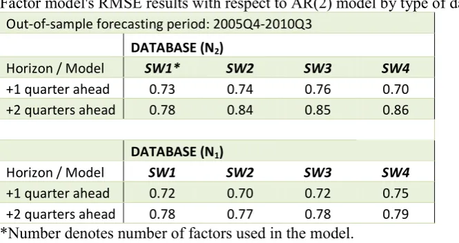
Results in Table 3 compare two types of specification. First, it compares results among specified
factor models with different number of factors. Second, Table 3 shows results for both types of
database specification. In addition, RMSE outcome determined in terms of AR(2) model results.
Thus a number below 1 assumes factor model’s better performance over AR(2) model. Results
suggest that on average full database tends to outperform reduced database.
& ' 1
Factor model's RMSE results with respect to AR(2) model by type of database
Out-of-sample forecasting period: 2005Q4-2010Q3
DATABASE (N2)
Horizon / Model SW1* SW2 SW3 SW4
+1 quarter ahead 0.73 0.74 0.76 0.70 +2 quarters ahead 0.78 0.84 0.85 0.86
DATABASE (N1)
Horizon / Model SW1 SW2 SW3 SW4
+1 quarter ahead 0.72 0.70 0.72 0.75 +2 quarters ahead 0.78 0.77 0.78 0.79
*Number denotes number of factors used in the model.
Table 4 shows outperformance of full database over reduced one. Positive number states by how
much full database outperforms another in terms of average percentage points of year on year
[image:8.595.83.416.474.650.2]8
& ' /
Comparison of RMSE of two databases by type of model
forecasting period: 2005Q4-2010Q3
Improvement (+) / Deterioration (-)
SW1 SW2 SW3 SW4
+1 quarter ahead 0.03 0.16 0.14 -0.18 +2 quarters ahead -0.05 0.53 0.50 0.48
According to the Table 4 forecasting 1 quarter ahead the full database N1 may outperform N2 on
about 0.15 percentage points assuming more correct model is chosen. In this case factor model with
2 factors behaves the best. Notably that for 2 quarters ahead improvement is more substantial. The
model specified with 2 factors accounts half percentage point of year on year growth rate.
We test ad hoc robustness check of the results by moving out of sample window back. Table 5
describes and compares factor models’ improvement results through the different out of sample
periods.
& ' 0
Forecasting improvement of factor models over the different out of sample periods
Improvement (+) / Deterioration (-)
+ 1 quarter ahead + 2 quarters ahead
Out-of-sample period SW1 SW2 SW3 SW4 SW1 SW2 SW3 SW4
2003Q4-2008Q3 -0.18 0.02 -0.03 0.04 -0.31 -0.04 -0.16 -0.05
2004Q1-2008Q4 -0.17 0.04 0.03 0.08 -0.29 -0.07 -0.12 -0.11
2004Q2-2009Q1 -0.18 0.15 0.12 0.04 -0.31 -0.03 0.00 -0.02
2004Q3-2009Q2 -0.22 0.14 0.14 0.05 -0.33 -0.01 0.02 0.02
2004Q4-2009Q3 -0.05 0.27 0.30 -0.10 -0.33 0.03 0.07 0.07
2005Q1-2009Q4 0.07 0.21 0.20 -0.16 -0.10 0.53 0.43 0.37
2005Q2-2010Q1 0.07 0.22 0.22 -0.16 0.01 0.61 0.59 0.49
2005Q3-2010Q2 0.02 0.15 0.12 -0.20 0.00 0.62 0.59 0.48
2005Q4-2010Q3 0.03 0.16 0.14 -0.18 -0.05 0.53 0.50 0.48
Starting with the out of sample time period of 2005Q4 2010Q3 we rolling back the fixed period
window and counts the outcome difference between database N1 and N2 as previously. We find that
appropriately specifying the model the constant improvement is observed forecasting 1 quarter
ahead. In turn, for two quarters horizon results more ambiguous. In the early years N1 database
wasn’t able to outperform N2 and forecasts accuracy is worse. On the other hand, in the later years
9
periods coincide with the deep economic crisis period is challenging and might raise the hypothesis
that more data still can capture more economic dynamics therefore forecasting accuracy may
improve.
According to this empirical study we conclude that additional information that contained in
disaggregated components of macroeconomic variables could be used to enhance Latvian GDP
forecasting accuracy. The efficiency gain improving forecasts is about 0.15 0.20 percentage points
of year on year quarterly growth for the forecasting horizon 1 quarter ahead, but for 2 quarters
ahead it’s about half percentage point. Robustness check shows that improvement is not constant for
the different models and forecasting horizons. While one can find stable outperformance pattern of
N1 over N2 for 1 quarter ahead forecasts, then for 2 quarters ahead there is the evidence that N1
unable to outperform N2 for any model in early out of sample periods.
Nonetheless results suggest that the use of disaggregated components does not provide the evidence
of huge efficiency loss or deterioration of the results due to disaggregated data. Moreover
appropriately specifying the model efficiency gain is positive.
Alternative way of research may be pursued toward finding schemes or criteria of weighting data
and/or even blocs of data in order to improve forecasting accuracy by using potentially valuable
disaggregated information.
Bessonovs A. (2010). Agregēta un dezagregēta faktoru modeļa pieeja IKP prognožu precizitātes
mērīšanā. Latvijas Universitātes raksti, 758 sējums. pp. 22 33.
Boivin, J., and Ng, S. (2006). Are more data always better for factor analysis? Journal of
Econometrics, 132:169 194.
Caggiano, G., Kapetanios., G., and Labhard, V., (2009). Are more data always better for factor
analysis? Results for the Euro Area, the six largest Euro Area countries and UK. ECB Working
10
Forni, M. and Reichlin, L., (1998). Let’s Get Real: a Factor Analytic Approach to Disaggregated
Business Cycle Dynamics, Review of Economic Studies 65, 453 473.
Forni, M., Hallin, M., Lippi, M. and Reichlin, L., (2001a). Coincident and Leading Indicators for the
Euro Area, Economic Journal 111, C82–85.
Johnson, R., A., Wichern D., W. (2007). Applied Multivariate Statistical Analysis. Sixth edition,
Pearson Prentice Hall.
Stock, J.,H., Watson, M.W., (1998). Diffusion Indexes. NBER Working Paper No. 6702.
Stock, J. H., Watson, M. W., (2002a). Macroeconomic Forecasting Using Diffusion Indexes.
Journal of Business & Economic Statistics, vol. 20, No. 2.
Stock, J. H., Watson, M. W., (2002b). Forecasting Using Principal Components from a Large
Number of Predictors. Journal of American Statistical Association, Vol. 97, No. 460, pp. 1167
Appendix 1 Data description
! " # $ % & & %' ' (( %
) * + , # $ %
) -( * + . #
) + ! ( "/ # (
" -( ! ! ! " ( ( (
, 0 ( -( ! ! ! " ( !'
. 1 ( % -( ! ! ! " (
" # % (
/ " # + % (
( ! ( ! " # ! (
1 ! ! ( ! "" #
1-( ! ! - ! ", #
-1 ! ( % ! ( ! ". # 2 ((
1-( ! ( % ! - ! ,/ # 2 ( 2 +' - ( & 2
1-( ! ( ! - ! , # ( ( ( ( (
, (
" , # ! ! (
, 3 ! , # (! ( (! ( (
. 3 - ! , # ( (
/ 4 ! , # ! * (
4 - ! ," #
! ,, # ( ' - ( ! % $ (
- ! ,. # ( ' ( (
5 ( % -( - ! ./ # $ (
# 6 ( ! ( . # ! % $ (
# 6 ( ! - ! . # ! ' *
" 0 ( . # ! ( $ (
, 0 - ! . #
. 0 ! ! . 7 !
. ( ! % $ (
/ ." 1 %' ' (( %
% 8 9 ( ! ( !
: + % ! ., # $ %
7 -( ! - ! .. #
% -( ! - ! // 1 %' ' (( %
1 ( % -( ! - !
-( ! - ! / # $ %
! / #
" / 1 %' ' (( %
, % ( ! ( ! "#
. # % % % / # $ %
/ 8; * ! % $ 9 / #
8; * ! % $ 9 / 1 %' ' (( %
< ! 8; * ! % $ 9 #
0! 8; * ! % $ 9 /" 1 ) = )>1' 7 )=' =5> 4 )5 7#7 :1 351=
0! ? $ ( 8; * ! % $ /, ' ' - (
7 ! 8; * ! % $ 9 /. (
3 8; * ! % $ 9 / ' ' &
" 1 % + * ( 2 ! ' (
, 1 ( % -( ! - ! ' (
( '
. % ( ' - (
/ 0 7 ! * (
( ' ( (! ' 2 $ ( (
" - ' ! ' 2 ! (
, - (
. ! ' 2 ! (
/ $ ( (
% ! 2 ' ( (
0 ( ' ' 2 (
" ! ! (( (
, ' ! $ ( ! ! ! (
. (
/ + ' 2 ( ( % (
"# " ( $ ( ' % (
% , > ( ! ( ' ' ! ( '
0 . ( ! ( ! ( (
Appendix 1 Data description
2 ' ( ' ' ' ( (
( $ ! # % &
2 ! 6 2 % ! 2
( ,. '
*! ./ = (
+ . : (
! . 3
7 ! ' + . ( ! * ! (
( . # (
" ) * @ . ! !
, 3 * ! . ! & !
. ) ! ' ." 2 ! ' ! ' + !
/ ! 2 ., < 2
@ ' 2 ' %' ! .. ( 2 & ( ( ( (
3 ! ' ! ! $ ( ! // -
-@ ! / 3 2 ' ! ' !
( / ) ' ( ' ' 2 (
/ ' ( ' ( ' 2 ! (
/
" 1 / # ! % ! (( & $ (
, ! / ( !
. # /" 7( (( & + 2 ! &
/ 15 @ 8 // A //9 /, #
11 @ 8 // A //9 /. '
= @ 8 // A //9 / = (
( ' : (
# $ % 3
# $ % & & %' ' ( ! * ! (
# # (
1 %' ' (( % ! !
" # 4 * ( ! &
, # 4 * " 2 ! ' ! ' +
. # 4 * > , < 2
/ # 4 * . ( 2 & ( ( ( (
# 4 * * / -
-# 4 * 1 % 3 2 ' ! ' !
' ) ' ( ' ' 2 (
5 ( % 8( 9 ' ( ' ( ' 2 ! (
B :
) & # ! % ! (( & $ (
# % 0 + # ( !
# % 0 + # " 7( (( & + 2 ! &
" # % 0 + # , #
, % $ % &
. ' ' ( ' * 8;9 .
-"/ ' ' ( ' ! * 8;9 /
-" '' ' ' * 8;9 1 (
-" ' ' ' ! * 8;9 0
" 1 8;9 1
-" 1 8;9 :
-" 8;9 1-
-" 8;9 4 -(
% ! " -(
"" 15 ?50> , 4
", 11 * & ( % &
". 11 * ( . 0 1-(
,/ 11 * ( / 0 (
* ! & 0 C
+ ' 0 C
, 7 ! ( 0 C >
, # % * ! 0 C
, # % * ! 0 C 7 !
, (
"
, 0! *
, # % * %
," # % %