Munich Personal RePEc Archive
Modeling employment dynamics with
state dependence and unobserved
heterogeneity
Prowse, Victoria
Department of Economics, Cornell University
10 April 2012
Online at
https://mpra.ub.uni-muenchen.de/38038/
Modeling Employment Dynamics with State Dependence and
Unobserved Heterogeneity
Victoria Prowse Department of Economics
Cornell University [email protected]
April 10, 2012
Abstract
We extend existing work on the dynamics of labor force participation by distinguishing between full-time and part-time employment and by allowing unobserved heterogeneity in the effects of previous employment outcomes, children and education on labor supply behavior. In addition, unobserved heterogeneity may feature autocorrelation and correlated random effects. Our results reveal significant variation in the effects of children and education on labor supply behavior. More-over, the omission of random coefficients and autocorrelation biases estimates of state dependencies. On average, temporary shocks that increase the rate of part-time employment lead subsequently to lower rates of non-employment than do shocks that temporarily increase the rate of full-time work.
Key Words: Discrete Labor Supply, Repeated Multinomial Choice; Maximum Simulated Likelihood Estimation.
1
Introduction
Labor supply behavior measured at the individual level displays a great deal of persistence (see, for example, Francesconi, 2002, and Booth et al., 1999). Persistence is observed both in participation decisions and in the hours of work of those in employment. In other words, we observe persistence on the extensive margin and on the intensive margin. It is well established, see for example Heck-man (1981a) and HeckHeck-man (1981b), that persistence in labor supply behavior can be generated by two different mechanisms. On one hand, individual characteristics may lead an individual to choose repeatedly the same employment state. Relevant characteristics consist of observables, such as ed-ucational qualifications and household structure variables, and unobservables including unobserved preferences and ability. Alternatively, persistence in labor supply behavior may arise from state de-pendencies, whereby an individual’s previous labor supply behavior has a causal effect on his or her current labor supply incentives. State dependencies may be generated by, for example, changes in preferences or constraints caused by previous working behavior. For the purpose of policy evaluation, it is critical to determine the relative contributions of state dependence and individual characteristics to the observed persistence in labor supply behavior. Indeed, if labor supply choices are driven entirely by observed or unobserved individual characteristics then the effect of a policy intervention, such as a wage subsidy or an in-work benefit, will cease the moment the policy is withdrawn. In contrast, if past labor market outcomes exert a causal effect on current labor supply behavior then the policy intervention will affect labor market outcomes beyond the duration of the policy.
There exist several studies of labor force participation dynamics. Notably, Heckman (1981a) studied the dynamics of women’s labor force participation decisions, while controlling for persistent unobserved individual characteristics. The results show that unobserved individual characteristics contribute significantly to the observed persistence in women’s labor force participation behavior but causal effects, or state dependencies, were also found to be present. A number of other studies report similar results, see inter alia, Booth et al. (1999) and Heckman and Willis (1977). Keane (1993) provided the first model of labor force participation with autocorrelated unobservables, while Hyslop (1999) extended the literature further by allowing both autocorrelated unobservables and correlated random effects, operationalized by including non-contemporaneous measures of observed individual characteristics, including measures of fertility at different points in the life-cycle. Keane and Sauer (2010) in turn extend the work of Hyslop (1999) by including classification error in the dependent variable and by introducing an alternative treatment of the initial conditions.
for estimates of state dependencies.
This paper makes two further contributions. First, we analyze the dynamics of individual labor supply in a multinomial choice framework, rather than the more often used binary choice model. While the generalization to a multinomial framework introduces concerns pertaining to identification and furthers computational complexity, this extension provides additional insight as it allows a study of the intertemporal dependencies associated with full-time and part-time employment. This mode of analysis therefore allows us to assess the likely employment trajectories induced by labor market policies that target specifically either full-time or part-time employment. Such results are of clear importance to policy makers who must decide how best to allocate limited resources. This analysis would not be possible using a binary model of labor market participation, such as the reduced form approach of Heckman (1981a) or the structural approach adopted by Eckstein and Wolpin (1989). Second, drawing on the unobserved heterogeneity in the effects of children on labor supply behavior permitted by our model, we are able to explore whether the relatively high rates of non-employment observed among women with young children are due to a common effect of young children on labor supply behavior or whether instead young children affect the labor supply behavior of only a subset of women.
The central econometric framework takes the form of a dynamic mixed multinomial logit model that features random coefficients, autocorrelated unobserved heterogeneity and time invariant unob-servables. We adopt a correlated random effects specification for the time invariant unobservables, and thereby permit unobservables to be correlated with individuals’ time varying characteristics, in-cluding children. In this respect, our specification is less restrictive than a standard random effects model, which would require that unobservables occur independently of individuals’ observed charac-teristics. Parameter estimates are obtained using Maximum Simulated Likelihood estimation. In a further round of empirical analysis, presented in Appendix C.1, we estimate two alternative model specifications, namely a model that attempts to proxy for possible sources of endogeneity and a model that is reduced form in the potentially endogenous variables, and we show that in both cases our key empirical findings continue to hold.
The empirical analysis is conducted using an eighteen year longitudinal sample taken from the British Household Panel Survey. The sample comprises married and cohabiting women and spans the years 1991-2009 inclusive. Three employment states are distinguished, namely full-time work, part-time work and non-employment. For the sample of women under consideration all three employment states are quantitatively important. Furthermore, there is a growing literature that documents the relatively low status of part-time jobs in the United Kingdom; notably Connolly and Gregory (2008) and Manning and Petrongolo (2008) show that part-time jobs are typically poorly paid and are con-centrated in menial occupations. Within the context of this literature it is important to establish whether part-time jobs are also associated with lower labor market attachment than full-time jobs.
work. Due to the asymmetric nature of the cross-state dependencies and the higher own-state depen-dence in part-time employment as compared to full-time employment, on average, temporary shocks that increase the rate of part-time employment lead subsequently to lower rates of non-employment than do shocks that temporarily increase the rate of full-time work. For women with young children we find that full-time employment provides a significant stepping-stone into part-time employment. However the reverse is not true; for women with young children part-time employment does not have a causal effect on subsequent full-time employment.
Our results further show significant, additional, variation in preferences for full-time and part-time work, relative to non-employment, among women with young children. We explore the implications of this variation for employment dynamics following the birth of a child. Our results show that the birth of a child is not associated with an increased likelihood of non-employment for women who have a high unobserved preference for full-time work in the event that they have a young child. Thus, the high rates of non-employment among women with children are due to changes in labor supply behavior among a subset of women with children, specifically those women who have a low unobserved preference for full-time work in the event that they have a young child.
Irrespective of the assumed distribution of the unobservables, we find that significant positive own-state dependencies are present in both full-time and part-time work. This result is in line with existing work on dynamic labor supply including Keane (1993) and Hyslop (1999). A comparison of our results across the different specifications of unobservables reveals that estimates of state dependencies are sensitive to the assumed distribution of the unobservables. As has been frequently found in studies of labor force participation, state dependencies are overestimated if persistent unobservables are ignored. Less predictably, the estimated state dependence in full-time employment tends to increase as the distribution of the unobservables is generalized from a specification allowing time invariant random intercepts to more general specifications allowing autocorrelated unobservables and random coefficients. We conclude that estimating dynamic labor supply models and ignoring autocorrelation and variation in the effects of observed individual characteristics on labor supply behavior may bias significantly estimates of the long-term effectiveness of labor market policies. The biases induced by ignoring autocorrelation or variation in the effects of observed individual characteristic pertain predominantly to the long-run effects of policies that facilitate full-time, rather than part-time, work. The next section outlines a model that describes an individual’s choice between full-time employ-ment, part-time employment and non-employment. Section 3 introduces a dynamic mixed multinomial logit model of labor supply behavior. Section 4 provides an overview of the British Household Panel Survey, and summarizes the main features of the estimation sample. Section 5 contains the results, including comparisons of estimated state dependencies as implied by models that feature different assumptions concerning the distribution of the unobservables. Section 6 concludes. The appendices can be found within the accompanying Supplementary Materials.
2
A Dynamic Multi-state Labor Supply Model
employment, part-time employment and non-employment. The model proceeds as follows. In year t
individualichooses between full-time employment (f), part-time employment (p) and non-employment (n) so as to maximize her current payoff. The individual receives a payoff Vj(Ω
i,t−1, Xi,t, ϱi,j,t) if she chooses employment statejat timetforj=f, p, n. Payoffs are functions of the relevant elements of the individual’s employment history, Ωi,t−1, individual characteristics observed by both the individual and
the econometrician, denoted Xi,t and henceforth referred to as explanatory variables, and individual characteristics that are known to the individual but which are unobserved to the econometrician, denoted ϱi,j,t for j = f, p, n. The variables Ωi,t−1, Xi,t and ϱi,j,t may be vectors. Conditional on observed characteristics and the individual’s employment history, optimizing behavior on the part of the individual implies the following labor supply probabilities
Pi,f,t(Ωi,t−1, Xi,t) = P (
Vf(Ω
i,t−1, Xi,t, ϱi,f,t)≥Vp(Ωi,t−1, Xi,t, ϱi,p,t)
Ωi,t−1, Xi,t
Vf(Ω
i,t−1, Xi,t, ϱi,f,t)≥Vn(Ωi,t−1, Xi,t, ϱi,n,t)
)
, (1a)
Pi,p,t(Ωi,t−1, Xi,t) = P (
Vp(Ω
i,t−1, Xi,t, ϱi,p,t)> Vf(Ωi,t−1, Xi,t, ϱi,f,t)
Ωi,t−1, Xi,t
Vp(Ω
i,t−1, Xi,t, ϱi,p,t)≥Vn(Ωi,t−1, Xi,t, ϱi,n,t)
)
, (1b)
Pi,n,t(Ωi,t−1, Xi,t) = P (
Vn(Ω
i,t−1, Xi,t, ϱi,n,t)> Vf(Ωi,t−1, Xi,t, ϱi,f,t)
Ωi,t−1, Xi,t
Vn(Ω
i,t−1, Xi,t, ϱi,n,t)> Vp(Ωi,t−1, Xi,t, ϱi,p,t)
)
, (1c)
where Pi,j,t(Ωi,t−1, Xi,t) is the probability of individual ichoosing employment state j at time t and P() denotes a probability.
The term “payoff” in this context refers to the individual’s utility associated with a particular employment state, taking into account any costs and benefits, as well as the income, associated with the employment state. Payoffs will depend on both the current period rewards to contemporaneous labor supply choices and, in the event that the individual is forward looking, the expected future benefits to current actions, including higher future wages arising from positive wage-based rewards to experience (see, for example, Eckstein and Wolpin, 1989; Francesconi, 2002).
The above formulation is sufficiently general to allow dependencies between an individual’s past and current labor supply decisions due to habit formation in labor supply behavior (Bover, 1991; Kubin and Prinz, 2002; Woittiez and Kapteyn, 1998), wage based rewards for human capital accumulated via labor market experience (Altug and Miller, 1998; Eckstein and Wolpin, 1989; Imai and Keane, 2004; Wolpin, 1992) and job search costs (Heckman and MaCurdy, 1980; Hyslop, 1999). Job search costs generate dependencies between labor supply choices in consecutive years, while habit formation and the accumulation of human capital have the potential to create dependencies in labor supply behavior spanning several years.
3
Estimation Strategy
The central econometric framework takes the form of a dynamic mixed multinomial logit model. Such a model is obtained by adopting a specification for the payoff functions appearing in the above la-bor supply probabilities and then placing appropriate distributional assumptions on the unobserved individual characteristics. This section proceeds by discussing the specification of payoffs, the deriva-tion of the likelihood funcderiva-tion, and issues surrounding identificaderiva-tion. Finally, the chosen empirical specification is presented together with the proposed Maximum Likelihood estimation method.
3.1 Specification of Payoffs
An examination of Equations (1a)-(1c) reveals that labor supply probabilities can be expressed in terms of the two indices Vf(Ω
i,t−1, Xi,t, ϱi,f,t) −Vn(Ωi,t−1, Xi,t, ϱi,n,t) and Vp(Ωi,t−1, Xi,t, ϱi,p,t) − Vn(Ωi,t−1, Xi,t, ϱi,n,t). (The third index Vf(Ωi,t−1, Xi,t, ϱi,f,t)−Vp(Ωi,t−1, Xi,t, ϱi,p,t) is redundant as it is equal to the difference between the other two indices.) The following specification is adopted
Vj(Ωi,t−1, Xi,t, ϱi,j,t)−Vn(Ωi,t−1, Xi,t, ϱi,n,t) = Ωi,t−1γj+Xi,tbj+hj(Ωi,t−1, Xi,t, ϱi,j,t) for j=f, p, (2)
where γj and bj for j = f, p are suitably dimensioned vectors of unknown parameters. The first two terms on the right hand side of the above represent the observed components of the individual’s payoff from statej forj =f, prelative to non-employment, while hj(Ωi,t−1, Xi,t, ϱi,j,t) forj=f, pare functions that describe the components of the individual’s payoffs from full-time and part-time work, relative to non-employment, that arise from the presence of the unobserved individual characteristics. The coefficient vectors bf and bp appearing in Equation (2) thus measure the marginal effects of the individual characteristics in Xi,t, such as education and household structure variables, on the observed components of the individual’s payoffs from, respectively, full-time work and part-time work relative to her payoff from non-employment. Meanwhile, the coefficient vectors γf and γp in Equation (2) measure the marginal effects of the individual’s employment history, Ωi,t−1, on the
observed components of her payoffs from, respectively, full-time work and part-time work relative to her payoff from non-employment. State dependencies are present if any elements of γf or γp are different from zero. The econometric analysis is conducted using panel data where information about an individual’s employment history is restricted to the duration of the individual’s presence in the panel. Thus, prior to estimation, restrictions on the specification of Ωi,t−1 are required. In this study
attention is restricted to the case where only the individual’s labor market outcomes in the past two years affect her payoffs in the current year. Specifically Ωi,t−1 = [Yi,f,t−1, Yi,p,t−1, Yi,f,t−2, Yi,p,t−2],
whereYi,j,t is an indicator taking the value one if individualiwas in employment statejat timetand zero otherwise. Suppose labor market outcomes are observed in yearst= 1, ..., T. Equation (2) then holds fort= 3, ..., T. This specification should not be overly restrictive as the strongest intertemporal dependencies in labor supply incentives are likely to occur over short time horizons.
state-specific variables, such as wages or measures of occupational status, because such quantities are unobserved for all employment states not chosen by the individual at time t. Instead, Xi,t includes variables that are generally deemed to be the underlying determinants of payoff-relevant employment state-specific outcomes. In consequence, the posited specification of payoffs is such that the financial incentives associated with employment choices are not modeled directly, i.e., income does not appear directly in the payoffs. One obvious limitation of this approach is that we are unable to determine the employment effect of a policy that changes the financial incentives associated with either employment or non-employment, for example a tax reform. However, this specification is adequate here as the focus of our study is on the implications of assumptions regarding the distribution of unobservables for estimates of state dependencies, rather than the behavioral effect of a specific policy intervention. An initial conditions problem arises when estimating this model. Given the dynamic structure of the model and the above described specification of the individual’s employment history, Ωi,t−1,
the individual’s employment outcome in the yeart= 1 depends on her employment outcomes in the years t = 0 and t = −1, which are unobserved to the econometrician. Likewise, the individual’s employment outcome in the year t = 2 depends on her unobserved employment outcome in the year t = 0. Therefore, employment outcomes in the years t = 1 and t= 2, referred to as the initial conditions and denotedICi, cannot be modeled in the same way as subsequent employment outcomes. When estimating the parameters of the above model, we adopt the treatment of the initial conditions proposed by Wooldridge (2005). According to this approach, the distribution of the unobservables and individual likelihood contributions are defined conditional on the initial conditions. The Wooldridge (2005) approach to the initial conditions problem provides a computational advantage, relative to the approach of Heckman (1981b), in the form of reducing the number of unknown parameters. We explain immediately below how we accommodate a dependence of the unobservables on the initial conditions.
The unobserved characteristics ϱi,j,t for j = f, p are henceforth taken to represent unobserved characteristics that affect the difference between the individual’s payoff from employment state j
and her payoff from non-employment. In the econometric analysis, we adopt a correlated random effects specification. Specifically, the adopted specification of the unobservables allows time invariant random intercepts, autocorrelated unobservables and time invariant random coefficients. Furthermore, we allow the time invariant random intercepts to be correlated with time varying observed individual characteristics and the initial conditions. Mathematically,
hj(Ωi,t−1, Xi,t, ϱi,j,t) = Ωi,t−1ωi,j+Wi,tπi,j+ζi,j,t+νi,j+ξi,f,t for j=f, p;t= 3, ..., T, (3)
where Wi,t denotes selected elements of Xi,t, andζi,f,t and ζi,p,t follow first order autoregressive pro-cesses
ζi,j,t =ρjζi,j,t−1+ςi,j,t for j=f, p; t= 3, ..., T. (4)
In the above ρj for j = f, p are autocorrelation coefficients and ({ξi,j,t, ςi,j,t}Tt=3, ωi,j, πi,j, νi,j) for j=f, pare unobserved individual characteristics.
and independently over time, and thus represent time varying shocks to individuals’ payoffs. The remaining unobserved individual characteristics consist of four distinct components: (i) ωi,f and ωi,p are the random components of the coefficients on the individual’s employment history, Ωi,t−1; (ii) πi,f and πi,p represent the random components of the coefficients on the explanatory variables, Wi,t; (iii) ζi,f,t andζi,p,t represent the autocorrelated random components of the employment state-specific intercepts; and (iv) νi,f and νi,p are the unobserved time invariant components of the employment state-specific intercepts.
We assume that, conditional onνi,j forj=f, p, the observed individual characteristicsXi,t and the initial conditionsICiare strictly exogenous. Mathematically, we require that ({ξi,j,t, ςi,j,t}Tt=3, ωi,j, πi,j) occur independently of Xi,s and ICi for all i, t, s and j. However, we capture the endogeneity of observed individual characteristics and the initial conditions by permitting a dependence of the time invariant unobserved components of the employment state-specific intercepts, that isνi,f and νi,p, on the individual’s observed characteristics and the initial conditions. Specifically, based on Chamberlain (1984), we adopt the following correlated random effects specification
νi,j =Ziλj+ICi(ϑj +ψi,j) +νei,j for j =f, p, (5)
whereZidenotes the vector of sample averages of individuali’s time varying characteristics, specifically children and unearned income, λj and ϑj for j =f, p are suitably dimensioned vectors of unknown parameters andψi,jforj=f, pare the random components of the coefficients on the initial conditions, ICi. In our empirical implementation, ICi consists of five variables indicating if the woman worked full-time, worked part-time or was non-employed in both t = 1 and t = 2, worked both full-time and part-time in her first two years in the sample or worked full-time and was non-employed in her first two years in the sample. According to Equation (5), the unobserved employment state-specific intercept νi,j is decomposed into a componentZiλj +ICi(ϑj+ψi,j), which reflects the contribution of observed individual characteristics and the initial conditions, and a second componenteνi,j which is unrelated to observables. We assume that both ψi,j and eνi,j occur independently of Xi,t and ICi for all i, tand j.
We do not attempt to estimate a fixed effects version of our model as this would introduce many largely unresolved issues. In particular, if any time invariant unobservables appearing in our model were treated as fixed effects then this would give rise to the well-known incidental parameters problem (Neyman and Scott, 1948), and lead the Maximum Likelihood Estimator to be biased, and inconsistent as the number of individuals goes to infinity with the number of time periods held fixed. Fern´andez-Val (2009) shows for a dynamic probit model that bias correction can reduce substantially finite sample bias (see Carro, 2007, and Hahn and Kuersteiner, 2004, for further results in this area). However, the empirical properties of bias corrected estimators have not been established in the current setting, where we have a non-linear, specifically multinomial, dynamic model with individual-specific intercepts and individual-specific coefficients on observed characteristics.
3.2 Derivation of the Likelihood Function
The following definitions are required prior to deriving individual i’s contribution to the likelihood. Define ϱi,j as ϱi,j,t stacked over t = 3, ..., T for j = f, p. Similarly, let Xi denote Xi,t stacked over
t= 3, ..., T. We useG(ϱi,f, ϱi,p|Xi, ICi) to denote the distribution of (ϱi,f, ϱi,p) conditional on observed
individual characteristics, Xi, and the initial conditions, ICi. Define the one by three dimensional vectors Af = (1,0,0), Ap = (0,1,0) and An = (0,0,1) and let Ai,t =Aj if individuali chose state j at timet forj=f, p, n. Additionally define the two by three dimensional matrixBi,t as follows
Bi,t =
(A′
p, A′n)′ ifYi,f,t = 1 (A′
f, A′n)′ ifYi,p,t = 1 for t= 3, ..., T. (A′
f, A′p)′ ifYi,n,t = 1
(6)
Lastly, let Vi,t denote Vj(Ωi,t−1, Xi,t, ϱi,j,t) stacked vertically overj=f, p, n. Individual i’s contribution to the likelihood takes the following form
Li =
∫
ϱi,f,ϱi,p
I(Ai,3Vi,3≥max{Bi,3Vi,3} ∩Ai,4Vi,4 ≥max{Bi,4Vi,4} ∩...
...∩Ai,TVi,T ≥max{Bi,TVi,T})dG(ϱi,f, ϱi,p|Xi, ICi), (7a)
= ∫
ϱi,f,ϱi,p
T ∏
t=3
I(Ai,tVi,t ≥max{Bi,tVi,t})dG(ϱi,f, ϱi,p|Xi, ICi), (7b)
whereI(.) is an indicator of whether the statement in parentheses is true and the integrals in the two above equations are over the entire support of (ϱi,f, ϱi,p).
3.3 Identification and the Distribution of Unobservables
constant does not change optimal behavior. In all that follows,G(ϱi,f, ϱi,p|Xi, ICi) is taken to be the distribution of the unobserved individual characteristics after the minimum normalizations required to ensure identification have been imposed.
The functions hj(Ωi,t−1, Xi,t, ϱi,j,t) for j = f, p and the distribution function G(ϱi,f, ϱi,p|Xi, ICi) together dictate both the structure of persistence in unobservables and the joint distribution of unob-servables occurring in a particular year. As discussed above, allowing persistence in unobunob-servables is necessary for determining correctly the nature of state dependence in labor supply behavior. Mean-while, Hausman and Wise (1978) show that estimates of marginal effects, substitution patterns and elasticities are not robust to the assumed intratemporal distribution of the unobservables. It is there-fore desirable to work with a flexible distribution of unobservables. However, even after imposing all necessary identifying scale and location normalizations, care is required when working with flexible forms of the above described structure of the unobservables. Indeed, unlike in the binary case, in the current multinomial labor supply model some of the more obvious, fully parametric, specifica-tions ofhj(Ωi,t−1, Xi,t, ϱi,j,t) forj =f, pand distribution of the unobserved individual characteristics, G(ϱi,f, ϱi,p|Xi, ICi), generate models that are identified purely by the functional form of the distri-bution of the unobserved individual characteristics, and therefore are nonparametrically unidentified. This results follows from Matzkin (1993), who considers identification of polychotomous choice mod-els in which neither the observable components of the payoff functions nor the distribution of the unobservable random terms are specified parametrically. A lack of nonparametric identification is conceptually unappealing. Furthermore, Keane (1992) presents Monte Carlo evidence that illustrates the very poor empirical performance of multinomial choice models in which parameters are identi-fied only by the functional form of the distribution of the unobservables. Thus, in the subsequent analysis, attention is restricted to model specifications in which the distribution of unobservables is nonparametrically identified.
The possibility of an absence of nonparametric identification can be understood by manipulating the individual likelihood contributions displayed above in Equation (7b). Letϱi,j,t denote ϱi,j,t net of the additive transient unobservableξi,j,tforj=f, pandt= 3, ..., T. Further, defineϱi,jasϱi,j,tstacked overt. In Section 3.1 we assumed that the pairs (ξi,f,t, ξi,p,t) fort= 3, ..., T are strictly exogenous and occur independently of the other unobservables and independently over time. Therefore
G(ϱi,f, ϱi,p|Xi, ICi) =Gϱ(ϱi,f, ϱi,p|Xi, ICi)
T ∏
t=3
Gtξ(ξi,f,t, ξi,p,t), (8)
where Gϱ(ϱi,f, ϱi,p|Xi, ICi) denotes the joint distribution of (ϱi,f, ϱi,p) conditional on Xi and ICi, and Gt
ξ(ξi,f,t, ξi,p,t) denotes the joint distribution of (ξi,f,t, ξi,p,t). Combining Equation (8) with Equa-tion (7b) gives
Li = ∫
ϱi,f,ϱi,p T ∏
t=3
∫
ξi,f,t,ξi,p,t
I(Ai,tVi,t ≥max{Bi,tVi,t}|ϱi,f, ϱi,p)dGtξ(ξi,f,t, ξi,p,t)
dGϱ(ϱi,f, ϱi,p|Xi, ICi). (9)
In a nonparametric setting each of the distribution functionsGt
varied independently of Gϱ(ϱi,f, ϱi,p|Xi, ICi). In other words there may be unknown parameters in
Gt
ξ(ξi,f,t, ξi,p,t) that affect the probability thatAi,tVi,t ≥max{Bi,tVi,t}conditional on the non-transient unobservables (ϱi,f, ϱi,p) but which do not enter Gϱ(ϱi,f, ϱi,p|Xi, ICi). In this case the bivariate dis-tribution functions, which appear in parentheses in Equation (9), are nonparametrically unidentified as the same observed variables affect both the probability thatAi,tVi,t > Bi,t,1Vi,t and the probability
thatAi,tVi,t > Bi,t,2Vi,t, whereBi,t,kfork= 1,2 denotes thekthrow ofBi,t. Obtaining models that are
nonparametrically identified thus requires that the distribution of the unobservables be restricted such thatGt
ξ(ξi,f,t, ξi,p,t) for t= 3, ..., T cannot be varied independently ofGϱ(ϱi,f, ϱi,p|Xi, ICi). Therefore, nonparametric identification requires that all unknown parameters appearing in the distribution of the unobservables must be identified from intertemporal rather than cross-sectional variation in behavior. In Section 3.4 below we explain how our adopted empirical specification ensures that we work with distributions of the unobservables that are nonparametrically identified.
Before proceeding, we make two further comments about identification. First, Equation (9) shows that the lack of nonparametric identification is related to the absence of employment state-specific explanatory variables. If, in contrast to the specification given in Equation (2), the payoffs included, for example, employment state-specific incomes or other characteristics of the employment states, parameters would, under appropriate regularity conditions, be nonparametrically identified (Harris and Keane, 1998, and Keane, 1992, provide further discussion of this issue). Second, we note that the lack of nonparametric identification is specific to discrete choice models with three or more alternatives; in the corresponding binary choice model nonparametric identification is less problematic as choice probabilities depend on a single index.
3.4 Empirical Specification
In accordance with the above described requirements for nonparametric identification, the time varying shocks to individuals’ payoffs (ξi,f,t, ξi,p,t) fort= 3, ..., T are assumed to have distributions that do not contain unknown parameters. In what follows,ξi,f,tandξi,p,tare defined respectively asϵi,f,t−ϵi,n,tand ϵi,p,t−ϵi,n,t for t= 3, ..., T whereϵi,j,t forj =f, p, n and are mutually independent and independent of {Xi,s}Ts=3 and ICi. Furthermore ϵi,j,t for j = f, p, n are assumed to have type I extreme value distributions. We note that one could instead assume ϵi,j,t ∼N(0,1). The latter assumption would also ensure that the distribution of the transient unobservables does not contain unknown parameters, but would yield a dynamic mixed multinomial probit model instead of a dynamic mixed multinomial logit model. The choice between a normal distribution and a type I extreme value distribution is not substantiative in this application as these two different distributional assumptions imply only a small difference in the distribution of the (suitably rescaled) error differences that appear in Equation (2).
independent over time and take the familiar multinomial logit form
Pi,j,t(Ωi,t−1, Xi,t, ϱi,f,t, ϱi,p,t) =
exp(Ωi,t−1γj+Xi,tbj+hj(Ωi,t−1, Xi,t, ϱi,j,t)) 1 +∑k=f,pexp(Ωi,t−1γk+Xi,tbk+hk(Ωi,t−1, Xi,t, ϱi,k,t))
forj=f, p;t= 3, ..., T, (10a)
Pi,n,t(Ωi,t−1, Xi,t, ϱi,f,t, ϱi,p,t) =
1
1 +∑k=f,pexp(Ωi,t−1γk+Xi,tbk+hk(Ωi,t−1, Xi,t, ϱi,k,t))
fort= 3, ..., T, (10b)
where, forj=f, pandt= 3, ..., T,hj(Ωi,t−1, Xi,t, ϱi,j,t) denoteshj(Ωi,t−1, Xi,t, ϱi,j,t) net of the additive transient unobservableξi,j,t. The expression for individual i’s likelihood contribution given above by Equation (7b) can be rewritten as follows
Li =
∫
ϱi,f,ϱi,p
T ∏
t=3 ∏
j=f,p,n
Pi,j,t(Ωi,t−1, Xi,t, ϱi,f,t, ϱi,p,t)Yi,j,tdGϱ(ϱi,f, ϱi,p|Xi, ICi). (11)
Nonparametric identification requires that all unknown parameters appearing in the distribution of the unobservables must be identified from intertemporal rather than cross-sectional variation in behavior. Consider the case where hj(Ωi,t−1, Xi,t, ϱi,j,t) allows only time invariant individual-specific random effects. In this case, two periods of observations subsequent to the initial conditions, i.e., four periods of observations including the two initial periods, is sufficient for nonparametric identification of G(ϱi,f, ϱi,p|Xi, ICi): with two periods of observations subsequent to the initial conditions the joint distribution of the non-transitory unobservables in adjacent time periods can be obtained, and with the restriction that non-transitory unobservables consist of time invariant random effects the distribution of the random effects is thus obtained (see Walker et al., 2007). By analogy, if hj(Ωi,t−1, Xi,t, ϱi,j,t) additionally allows autocorrelation in the employment state-specific intercepts then nonparametric identification ofG(ϱi,f, ϱi,p|Xi, ICi) requiresT ≥5; an extra year of observations is required in order to separate the autocorrelated and time invariant unobservables. The introduction of random coefficients does not require a longer panel for nonparametric identification provided that random coefficients on the time dummies and any other variables that, for all individuals, are non-zero in a maximum of one year between t= 3 and T are excluded. This ensures that all random coefficients with a distribution that contains unknown parameters affect payoffs in at least two years between t= 3 and t=T.
third specification we assume a distribution generated by a mixture of two normal distributions with different means and covariance matrices. The fourth specification allows the employment state-specific intercepts to contain time invariant components, as in the second specification, and autocorrelated components, where the autocorrelation processes are jointly normal and the initial conditions of the autocorrelation processes ensure stationary. The fifth specification allows time invariant individual effects, as in the second specification, and random coefficients on the individual’s previous employment outcomes, the initial conditions and selected explanatory variables. The two random coefficients on a particular variable, for example the kth elements of π
i,f and πi,p, are assumed to be jointly normally distributed with zero mean and an unrestricted covariance matrix, and all pairs of random coefficients are mutually independent and independent of the random components of the employment state-specific intercepts. Allowing correlations between all pairs of random coefficients leads to a prohibitively large number of parameters. The sixth specification is the most general specification under consideration and augments the fifth specification by permitting autocorrelation, as previously described, in the employment state-specific intercepts. The notes accompanying Table 3 provide further details concerning the implemented distributions of the unobservables.
We refrain from considering latent class models. According to this approach, each individual is one of a finite number of distinct types, and each type is characterized by a particular vector of unobserved attributes. Latent class models thus provide a means of including permanent unobservables but with-out the need to specify a particular distribution. However, such models quickly proliferate parameters as the number of types or latent attributes increases. Another alternative, nested models, have be used extensively in multinomial choice problems in order to capture cross-alternative correlations in unobservables, particularly in applications where the choice set is large. However, in the current appli-cation nested models do not provide a natural means of modeling the unobservables. In particular, the application of a nested model requires that choice alternatives be assigned to nests prior to estimation. However, given the choice alternatives of full-time work, part-time work and non-employment, there is no entirely plausible allocation of choice alternatives to nests. Indeed, there are reasons for grouping part-time employment with both full-time employment and non-employment. Finally, neither latent class models nor nested models can accommodate straightforwardly autocorrelation.
3.5 Estimation Methodology and Performance
involve 2(T −2) dimensional integrals. For two dimensional problems fast and accurate quadrature methods are available to evaluate the individual likelihood contributions (Geweke, 1996, provides a survey). However numerical methods are unable to evaluate the likelihood contributions with sufficient speed and accuracy to be effective in problems where the dimension of integration is greater than two (see Bhat, 2001; Hajivassiliou and Ruud, 1994). Consequently, in the context of the current applica-tion, numerical methods to evaluate the likelihood contributions are unavailable when unobservables feature random coefficients on several variables or whenT is moderately large and unobservables are autocorrelated.
For models where an analytic expression for the likelihood is unavailable we use simulation tech-niques to evaluate the likelihood contributions. Simulation methods replace the intractable integral in the likelihood function by a sum over likelihood functions evaluated at different draws from the distribution of unobserved heterogeneity. Let (ϱr
i,f, ϱri,p) denote the rth draw from the distribution G(ϱi,f, ϱi,p|Xi, ICi) for individual i. Individuali’s likelihood contribution is simulated as follows
Lsi = 1
R R ∑
r=1 T ∏
t=3 ∏
j=f,p,n
Pi,j,t(Ωi,t−1, Xi,t, ϱi,f,tr , ϱri,p,t)Yi,j,t. (12)
Continuing to assume independence over individuals, the simulated likelihood is the product of the simulated individual likelihood contributions for the sample members. Maximum Simulated Likelihood estimates are obtained by maximizing the log simulated likelihood function. By the strong law of large numbers the Maximum Simulated Likelihood estimates converge almost surely to the true parameters as R → ∞ and N → ∞. Moreover, if R increases at a fast enough rate relative to N, Maximum Simulated Likelihood estimation is asymptotically equivalent to Maximum Likelihood estimation. In particular, with pseudo random draws, √N /R→ 0 as N → ∞ is required (Hajivassiliou and Ruud, 1994).
In this application, the likelihood is simulated using antithetic variates rather than pseudo random draws. Antithetic variates are a variance reduction technique which reduces simulation noise by using draws from the distribution of the unobservables with more even coverage than pseudo random draws (see Train, 2003, for a description of the construction of antithetic variates). Hajivassiliou (1999) presents Monte Carlo evidence which shows that the use of antithetic variates in Maximum Simulated Likelihood problems approximately halves the number of draws required to obtain a given level of accuracy. We note that Halton draws are not appropriate in this application due to the high correlation, and therefore poor multidimensional coverage, of the draws which occurs in high dimensional problems, such as the one in hand. Indeed, Hess and Polak (2003) show that the poor multidimensional coverage of high dimensional Halton draws can cause serious problems in the estimation of models with high-dimensional integrals.
considera-tion. In summary, for a specification in which unobservables include random coefficients but exclude autocorrelated unobservables evaluation of the likelihood using 500 antithetic draws yields parameter estimates with tolerably small amounts of bias. A specification including autocorrelation displays a moderate amount of simulation bias when 500 or 2,000 antithetic draws are used, but biases are relatively small when estimation uses 5,000 antithetic draws. Therefore all of our empirical analysis uses 5,000 antithetic draws.
4
Data and Sample
The data source used for the empirical analysis is the British Household Panel Survey (BHPS). The BHPS is an ongoing annual panel survey that started in 1991 with a nationally representative sample of approximately 5,500 households in Great Britain. The sample used for analysis is a weakly balanced panel covering the years 1991 - 2008. We construct our sample such that each individual is present for exactly 13 years. Attention is restricted to married or cohabiting, non-retired women aged between 18 and 65 years. Single mothers and single adult households are therefore excluded from the sample. Women who satisfy the sample selection criteria for more than thirteen consecutive years enter our sample at a date randomly selected from those dates that provide at least thirteen consecutive obser-vations, and leave the sample after thirteen years. The final sample consists of 1,288 different women and 16,744 person-year observations. The previously described method for constructing the sample was chosen for three reasons. First, the weakly balanced panel structure allows us to employ the treat-ment of the initial conditions proposed by Wooldridge (2005) (see the final paragraph of this section for further discussion of this approach). Second, as noted above in Section 3.4, robust identification of the parameters of model specifications that feature both autocorrelation and time invariant random intercepts requires a minimum of five repeated observations. A panel length of thirteen observations per individual therefore provides a sufficient number of repeated observations to allow us to distinguish empirically the various sources of persistence in behavior. Third, random selection of the sample entry date for individuals who provide in excess of thirteen consecutive observations ensures that we have enough observations in each calender year to be able to control effectively for common time effects.
0
.01
.02
.03
.04
.05
Density
0 10 20 30 40 50 60
Weekly working hours
(a) Density of observed usual weekly working hours for women in employment.
0
20
40
60
80
Percentage
1 2 3 4 5 6 7 8 9 10 11 12
Years after reference date
Full−time Part−time Non−emp.
(b) Labor market outcomes of women who were work-ing full-timetyears previously.
0
20
40
60
80
Percentage
1 2 3 4 5 6 7 8 9 10 11 12
Years after reference date
Full−time Part−time Non−emp.
(c) Labor market outcomes of women who were working part-timetyears previously.
0
20
40
60
80
Percentage
1 2 3 4 5 6 7 8 9 10 11 12
Years after reference date
Full−time Part−time Non−emp.
(d) Labor market outcomes of women who were non-employedtyears previously.
[image:17.595.59.539.59.429.2]Notes: The sample used to construct Figure 1(a) has been truncated at 60 hours per week which excludes 0.5% of the observations.
Figure 1: Density of observed hours of work, and observed persistence in employment outcomes.
the current year. Similarly, approximately 80% of women who were working part-time or who were non-employed one year previously are in the same employment state in the current year. There is also evidence of persistence over a longer time horizon. For example, around 55% of women who were working full-time 12 years previously are currently in full-time work. The corresponding figures for part-time work and non-employment are 50% and 46% respectively.
contains further details concerning the explanatory variables.
Finally, we comment on the nexus of our weakly balanced panel structure, the use of the Wooldridge (2005) approach to the initial conditions and the adopted correlated random effects specification. Given our weakly balanced panel structure, all individuals are observed for exactly thirteen consecutive years, however individuals differ in the date at which they enter the sample, e.g., some individuals are observed from 1991-2003 inclusive, while others are observed from 1995-2007. The construction of Equation (5) assumes implicitly that the link between the random intercepts, νi,j for j = f, p, and individual-specific averages of time varying characteristics, Zi, and the initial conditions, ICi is common across individuals. Therefore, in the context of our weakly balanced panel structure we require that the relationship between the random interceptsνi,j forj=f, pand the relevant observables does not depend on the specific years in which the individual was present in the sample.
5
Results
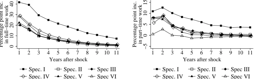
The dynamic mixed multinomial logit model is estimated with six different specifications of unobserved individual characteristics, as described above in Section 3.4. The parameter estimates and average marginal effects obtained from Specification VI, the most general specification under consideration, are discussed in Section 5.1. In sections 5.2 and 5.3 we explore respectively the nature of state dependence in women’s labor supply behavior and the extent of any heterogeneity in labor supply dynamics following the birth of a child, again based on Specification VI. In Section 5.4 we investigate the importance of allowing autocorrelation and random coefficients by making comparisons of the results obtained from Specification IV with those obtained from Specifications I-V, which impose more restrictive distributions of unobservables.
5.1 Parameter Estimates and Average Marginal Effects
Specification VI is the most general specification under consideration. This specification allows ran-dom intercepts with both time invariant and autocorrelated components, and time invariant ranran-dom coefficients. The time invariant components of the random intercepts are allowed to be correlated with the individual’s observed characteristics and the initial conditions. The time invariant random coefficients appear on the indicator of having a degree, the indicator of the woman’s youngest child being aged under one year, and on the variables describing the initial conditions. Experimentation with various specifications of the random coefficients revealed that there are no random coefficients with significant amounts of variation on any other explanatory variables.
Variable Year
1991 1992 1993 1994 1995 1996 1997 1998 1999 2000 2001 2002 2003 2004 2005 2006 2007 2008 Highest Educational Qualification:
DEGREE 0.13 0.13 0.14 0.14 0.15 0.16 0.16 0.16 0.16 0.16 0.17 0.17 0.17 0.18 0.19 0.19 0.19 0.18 HIGHER QUAL. BELOW DEGREE LEVEL 0.15 0.16 0.16 0.18 0.18 0.20 0.21 0.23 0.24 0.26 0.28 0.29 0.31 0.32 0.33 0.36 0.38 0.41 A LEVELS 0.10 0.11 0.10 0.11 0.12 0.12 0.12 0.11 0.11 0.11 0.10 0.10 0.10 0.11 0.10 0.10 0.11 0.08 GCSES 0.27 0.27 0.27 0.26 0.26 0.25 0.25 0.24 0.23 0.22 0.21 0.21 0.20 0.19 0.19 0.17 0.16 0.17
UNEARNED INCOME 13.36 12.56 12.16 11.99 12.12 12.39 12.75 12.98 13.51 13.61 13.98 14.18 14.32 14.40 16.08 16.59 17.63 17.64 AGE 36.09 36.54 36.71 37.26 37.36 37.48 38.48 39.48 40.46 41.49 42.48 43.47 44.48 44.52 44.52 44.85 44.86 45.67 YOUNGEST CH. 0-1 YEARS 0.08 0.12 0.05 0.07 0.05 0.06 0.06 0.06 0.04 0.04 0.04 0.04 0.03 0.03 0.02 0.02 0.03 0.01 YOUNGEST CH. 1-2 YEARS 0.14 0.13 0.13 0.10 0.13 0.11 0.10 0.10 0.10 0.10 0.08 0.08 0.07 0.07 0.07 0.06 0.04 0.06 YOUNGEST CH. 3-4 YEARS 0.06 0.06 0.10 0.10 0.08 0.08 0.10 0.09 0.08 0.08 0.08 0.07 0.06 0.07 0.09 0.08 0.10 0.07 YOUNGEST CH. 5-6 YEARS 0.04 0.04 0.06 0.08 0.07 0.07 0.07 0.07 0.08 0.08 0.06 0.06 0.06 0.06 0.05 0.08 0.10 0.08 YOUNGEST CH. 7-11 YEARS 0.15 0.15 0.13 0.14 0.14 0.13 0.13 0.14 0.15 0.15 0.16 0.17 0.16 0.17 0.19 0.17 0.17 0.21 YOUNGEST CH. 12-15 YEARS 0.13 0.11 0.11 0.10 0.10 0.09 0.10 0.10 0.10 0.10 0.11 0.10 0.11 0.11 0.11 0.13 0.12 0.13 PROTESTANT 0.66 0.65 0.63 0.65 0.64 0.63 0.63 0.63 0.63 0.63 0.63 0.63 0.63 0.62 0.61 0.63 0.59 0.57 CATHOLIC 0.12 0.12 0.13 0.13 0.13 0.12 0.12 0.12 0.12 0.12 0.12 0.12 0.12 0.12 0.12 0.11 0.11 0.10
FAMILY VALUES I
Family suffers when woman works full-time 0.32 0.34 0.34 0.34 0.32 0.32 0.33 0.33 0.34 0.34 0.32 0.32 0.31 0.32 0.34 0.36 0.34 0.27
FAMILY VALUES II
Husband and wife should contribute to household income 0.43 0.44 0.44 0.45 0.42 0.43 0.42 0.42 0.40 0.40 0.40 0.40 0.37 0.36 0.35 0.37 0.36 0.36
[image:19.595.115.770.127.352.2]Observations 272 501 696 869 1055 1288 1288 1288 1288 1288 1288 1288 1288 1016 787 592 419 233 Notes: DEGREE, HIGHER QUAL. BELOW DEGREE LEVEL, A LEVELS and GCSES are indicators of a woman’s highest qualification being, respectively, a university degree, a non-degree level higher qualification, A levels or equivalent qualifications (A Levels are usually taken at age 18 years) or grade A-C GCSEs or equivalent qualifications (GCSEs are usually taken at age 16 years). UNEARNED INCOME refers to a woman’s annual net unearned income including her partner’s income expressed in pounds sterling and deflated to year 1991 prices using the Retail Price Index. AGE is the woman’s age in years. YOUNGEST CH.a−bYEARS is an indicator of the youngest child in the household being aged betweenaandbyears at 2 months after the date of the annual survey. PROTESTANT and CATHOLIC are indicators of the woman’s religious denomination being, respectively, protestant and catholic. FAMILY VALUES I is an indicator that takes the value one if the woman agrees with the statement “all in all, family life suffers when the woman has a full-time job” and zero otherwise. FAMILY VALUES II is an indicator that takes the value one if the woman agrees with the statement “both husband and wife should contribute to the household income” and zero otherwise.
Table 1: Sample means of the explanatory variables in years 1991-2008.
qualifications. Young children have a strong negative effects on the probabilities of both full-time and part-time employment. Specifically, women whose youngest child is aged one year or under are on average 34.36(1.90) percentage points less likely to be working full-time and 9.02(2.88) percentage points less likely to be working part-time than otherwise identical women without children. The effect of children on a woman’s probability of engaging in full-time work decreases quickly as the age of the woman’s youngest child increases, while a youngest child aged between 1 and 7 years has a significant positive effect the probability of part-time employment.
We find that unearned income has a negative effect on the probability of full-time work and on the probability of part-time work, but neither effect is significant. This result is not surprising as, via the correlated random effects specification (see Equation (5)), the individual-specific average of unearned income is included in the payoffs, in addition to the contemporaneous value of unearned income. Therefore, the marginal effects of unearned income reported for Specification VI in Table 4 refer to the effect of transitory, rather than permanent, unearned income. Consistent with the theoretically negative effect of life-cycle unearned income on labor supply, the coefficients on the individual-level average of unearned income in the payoffs from full-time and part-time work (not reported) are both significantly negative (based on Specification VI, p values are 0.001 and 0.016 for the coefficients on individual-level average income in the payoffs from full-time and part-time employment, andp= 0.001 for the joint hypotheses that both coefficient equal zero).
The results for Specification VI in Table 4 further show that, on average over the sampled women, working full-time rather than being non-employed in the previous year increases the probability of working full-time in the current year by 43.93(4.39) percentage points. Similarly, working part-time rather than being non-employed increases the probability of working part-time in the current year by 23.40(2.93) percentage points. These results confirm the presence of significant state dependence in women’s labor supply behavior. The nature of the intertemporal dependencies in labor supply behavior is explored in further detail below in Section 5.2.
Variable Spec. I Spec. II Spec. III Spec. IV Spec. V Spec. VI
f p f p f p f p f p f p
Yi,f,t−2 2.35
(0.16) (01..1712) (01..5718) (00..7114) (01..6318) (00..7214) (02..0840) (01..1024) (01..5524) (00..6919) (02..3042) (01..1528)
Yi,p,t−2 1.11
(0.15) (01..3609) (00..7617) (00..9111) (00..8217) (00..9111) (01..0127) (01..1420) (00..8321) (00..9115) (01..0829) (01..0920)
Yi,f,t−1 4.09
(0.16) (01..7212) (03..1219) (01..1814) (03..1619) (01..2214) (04..5068) (01..6547) (03..3725) (01..2521) (05..2566) (01..3740)
Yi,p,t−1 2.47
(0.14) (03..0709) (01..9617) (02..5911) (01..9917) (02..6011) (02..7051) (02..9137) (01..8520) (02..6513) (02..7146) (02..9031)
Highest Educational Qualification:
DEGREE 0.61
(0.13) (00..2411) (00..9424) (00..3719) (00..9324) (00..3419) (01..0727) (00..4521) (00..9027) (00..4122) (01..1235) (00..5027)
HIGHER QUAL. BELOW DEGREE LEVEL 0.55
(0.11) (00..4209) (00..9219) (00..6715) (00..9119) (00..6515) (00..9722) (00..7318) (00..8622) (00..7119) (01..1029) (00..8824)
A LEVELS 0.42
(0.14) (00..2313) (00..7724) (00..4420) (00..7824) (00..4320) (00..8727) (00..5022) (00..6926) (00..4423) (00..7934) (00..5228)
GCSES 0.37
(0.11) (00..2509) (00..5519) (00..3815) (00..5519) (00..3615) (00..5722) (00..4117) (00..4622) (00..3819) (00..6228) (00..4923)
UNEARNED INCOME/100 −1.47
(0.28)
−0.67
(0.26)
−0.56
(0.49)
−0.39
(0.49)
−0.56
(0.49)
−0.35
(0.50)
−0.64
(0.59)
−0.33
(0.55)
−0.65
(0.54)
−0.52
(0.53)
−0.96
(0.72)
−0.63
(0.64)
AGE/10 −0.88
(0.23) 0
.16
(0.23) −(01..5445) 0
.07
(0.39) −(01..5044) 0
.11
(0.39) −(01..50)62 0
.08
(0.41) −(01..49)82
−0.19
(0.43)
−2.39
(0.63)
−0.30
(0.51)
YOUNGEST CH. 0-1 YEAR −4.42
(0.16)
−2.28
(0.17)
−5.28
(0.25)
−2.72
(0.23)
−5.19
(0.25)
−2.66
(0.23)
−5.94
(0.70)
−2.91
(0.49)
−6.08
(0.43)
−2.97
(0.30)
−8.35
(0.85)
−3.95
(0.55)
YOUNGEST CH. 1-2 YEARS −0.55
(0.16) 0
.72
(0.15) −(01..6726) 0
.24
(0.22) −(01..5826) 0
.29
(0.23) −(01..34)46 0
.38
(0.25) −(01..28)88 0
.07
(0.24) −(02..43)54
−0.32
(0.31)
YOUNGEST CH. 3-4 YEARS −0.37
(0.18)
0.53
(0.15) −(01..4227)
0.19
(0.23) −(01..3527)
0.25
(0.23) −(01..34)23
0.32
(0.25) −(01..29)61
0.04
(0.25) −(02..42)24
−0.26
(0.30)
YOUNGEST CH. 5-6 YEARS 0.21
(0.18) (00..15)77 −(00..7226) 0
.59
(0.22) −(00..6626) 0
.64
(0.22) −(00..31)45 0
.75
(0.24) −(00..28)85 0
.49
(0.23) −(01..38)26 0
.31
(0.28)
YOUNGEST CH. 7-11 YEARS 0.19
(0.14) (00..4113) −(00..4622)
0.41
(0.20) −(00..4122)
0.44
(0.20) −(00..26)29
0.49
(0.22) −(00..24)54
0.34
(0.21) −(00..32)81
0.25
(0.25)
YOUNGEST CH. 12-15 YEAR 0.50
(0.16) (00..2614) (00..0821) (00..2718) (00..1321) (00..2918) (00..2324) (00..3320) (00..0222) (00..2219) (00..0129) (00..2323)
INTERCEPT −3.11
(0.33)
−2.62
(0.31)
−2.70
(0.50)
−2.40
(0.43)
−2.72
(0.58)
−2.77
(1.00)
−3.27
(0.65)
−2.54
(0.50)
−2.41
(0.55)
−2.20
(0.47)
−3.79
(0.78) 1
.84
(0.48)
Log Likelihood -6913.55 -6825.68 -6823.30 -6822.82 -6791.79 -6778.67 Pseudo R2 54.25% 54.82% 54.84 % 54.84% 55.05% 55.13%
AIC 13987.09 13845.35 13852.60 13849.65 13813.57 13797.35 BIC 14591.79 14578.55 14631.15 14620.64 14682.83 14704.39 Joint Significance of
- p= 0.000 p= 0.000 p= 0.019 p= 0.000 p= 0.001 Correlated Random Effects
Notes: Standard errors in parentheses. Estimates of the coefficients on the year dummies and the initial conditions are omitted. Columns headedf
andpcontain the coefficients describing payoffs from respective full-time employment and part-time employment. AIC=-2Log likelihood+2Parameters; BIC=-2Log likelihood+ ln(N T)Parameters; Pseudo R2=1-Restricted Log likelhood/Unrestrcited Log likelihood. See notes to Table 1 for variable
definitions.
[image:21.595.132.749.66.457.2]Spec. II Spec. III Spec. IV Spec. V Spec. VI
ΣIntercept 1
2.61 (0.39) .
1.43 (0.25) (01..2222)
2.81 (0.62) .
1.52 (1.07) (11..2159)
2.75 (0.65) .
1.55 (0.44) (01..2836)
2.57 (0.47) .
1.54 (0.30) (01..0326)
4.53 (0.97) .
2.68 (0.62) (01..8448)
ΣIntercept 2
1.65 (0.52) .
0.88 (0.28) (00..4764)
µ2
0.94 (0.94) 1.06 (1.06)
α 0.63
(0.03)
ρf −0.16
(0.19)
−0.12 (0.10)
ρp 0.12
(0.29) (00..3119) Σζ
2.39 (1.59) .
0.96 (0.04) (00..7383)
5.64 (1.87) .
0.89 (0.11) (01..3275)
ΣYi,f,t−2
0.30 (0.42) .
0.02 (0.23) (00..0003)
0.66 (0.64) .
0.20 (0.39) (00..0723)
ΣYi,p,t−2
0.18 (0.37) .
0.25 (0.33) (00..3431)
0.23 (0.56) .
0.18 (0.41) (00..2334)
ΣYi,f,t−1
0.63 (0.49) .
0.68 (0.47) (01..1260)
0.02 (0.19) .
0.09 (0.39) (00..5059)
ΣYi,p,t−1
0.06 (0.15) .
−0.13 (0.11) 0
.28 (0.24)
0.06 (0.18) .
−0.14 (0.17) 0
.34 (0.32)
ΣDEGREE
0.53 (0.72) .
0.68 (0.54) (01..2153)
0.76 (0.77) .
1.15 (0.82) (01..7465)
ΣCHILD
7.71 (2.88) .
4.42 (1.68) (12..5335)
13.47 (5.43) .
7.42 (2.94) (24..2804)
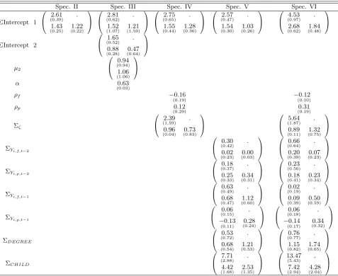
Notes: Standard errors in parentheses. Specification I has no unknown parameters in the distribution of the unobserv-ables. In Specifications II and IV-VI, ΣIntercept 1 is the covariance matrix of the time invariant components of the random intercepts. Specification III has time invariant random intercepts with a distribution obtained from the mixture of two bivariate normal distributions: with probabilityαthe random intercepts have mean zero and variance ΣIntercept 1 and with probability (1−α) the random intercepts have meanµ2 and variance ΣIntercept 2. In specifications al-lowing autocorrelation in the random intercepts,ρf andρpare the first order autocorrelation coefficients and Σζ is the
covariance matrix of the innovations in the autoregressive processes. ΣDEGREEand ΣCHILDare the covariance matrices
[image:22.595.62.540.55.445.2]of the random coefficients on the indicated variables. The covariance matrices of the random coefficients on the initial conditions in Specifications V and VI are not reported, and the coefficients associated with the correlated random effects are omitted.
Table 3: Estimates of parameters appearing in the distribution of unobservables for Specifications II-VI of the dynamic mixed multinomial logit model.
the time-invariant random intercepts and observed individual characteristics.
5.2 Labor Supply following Employment Shocks
Variable Spec. I Spec. II Spec. III Spec. IV Spec. V Spec. VI
f p f p f p f p f p f p
nt−1→ft−1 52.39
(2.27) −(18..87)62
32.47
(2.40) (22..4009) 33(3..79)07 −(28..89)80
42.38
(4.34) −13(3..70)82
34.22
(2.92) −11(2..31)06
43.93
(4.39) −21(3..90)69
nt−1→pt−1 4.95
(1.70) 39(1..72)88 −(10..79)35 1
.79
(2.05) (30..3037) 28(5..90)36 (23..6547) 27(2..73)71 −(22..4347) 29
.67
(3.30) (21..9432) 23(2..93)40
NO EDUC.→GCSES 1.57
(0.75) (00..5186) (12..6837) (11..3738) (12..8230) (10..7121) (12..0514) (11..2125) (12..5443) (11..0147) (12..1425) (11..6832)
NO EDUC.→A LEVELS 2.10
(0.90) (10..0204) (14..5475) (11..7553) (14..5858) −(10..57)10
4.00
(1.57) (10..2661) (14..1978) (10..2162) (13..1237) (11..0468)
NO EDUC.→HIGHER QUAL BELOW DEGREE LEVEL 2.03
(0.75) (01..3178) (14..2246) (11..4630) (14..2130) (11..6823) (13..3022) (12..1820) (13..9142) (12..1647) (13..1725) (12..9439)
NO EDUC.→DEGREE 3.73
(0.81) −(01..95)12
6.71
(1.68) (11..6860) (16..7169) −(12..53)31
6.17
(1.49) −(11..8346)
6.33
(1.75) −(11..5358)
5.47
(1.50) −(10..9653)
UNEARNED INCOME+£1000 −8.55
(2.00) 1
.12
(2.45) −(32..6984) 3
.84
(4.95) −(32..9344)
−0.46
(4.02)
−3.13
(3.70) 0
.28
(4.91) −(32..5556)
−1.92
(4.36)
−3.15
(3.68)
−1.36
(4.99)
AGE + 1 YEAR −0.21
(0.04)
0.19
(0.05) −(00..3907)
0.07
(0.08) −(00..3509)
0.28
(0.10) −(00..3808)
0.31
(0.09) −(00..3808)
0.23
(0.09) −(00..3708)
0.26
(0.09)
NO CHILDREN→CHILD AGED≤1 YEAR −31.87
(1.18)
−7.60
(2.13)
−35.28
(1.82)
1.82
(2.63) −35(2..87)28
−6.93
(3.14)
−33.36
(1.69)
−5.94
(2.49)
−35.26
(2.53)
−7.68
(5.60)
−34.36
(1.90)
−9.02
(2.88)
NO CHILDREN→1 YEAR<CHILD AGED≤2 YEARS −9.75
(1.12)
12.06
(1.30) −18(2..24)84
2.24
(2.50) −18(2..84)26
15.83
(3.80) −15(2..02)50
14.97
(2.15) −19(2..25)12
14.74
(2.39) −16(2..34)57
11.42
(2.69)
NO CHILDREN→2 YEAR<CHILD AGED≤4 YEARS −6.76
(1.33)
8.38
(1.44) −16(2..37)07
2.37
(2.59) −15(2..64)65
13.59
(3.42) −13(2..36)08
12.57
(2.56) −16(2..36)36
12.42
(2.49) −14(2..30)79
10.43
(2.49)
NO CHILDREN→4 YEAR<CHILD AGED≤7 YEARS −3.36
(1.11) 7
.15
(1.25) −12(2..02)23 2
.02
(2.12) −11(2..76)87 13
.39
(3.38) −(29..4416) 12
.15
(2.28) −12(2..09)43 12
.59
(2.21) −11(2..06)28 11
.03
(2.42)
NO CHILDREN→7 YEAR<CHILD AGED≤11 YEARS −1.04
(0.89)
3.23
(0.97) −(18..1581)
1.81
(1.76) −(27..6810)
8.74
(2.46) −(16..0775)
7.78
(1.88) −(18..1769)
8.27
(1.75) −(17..6179)
7.56
(1.96)
NO CHILDREN→11 YEAR<CHILD AGED≤16 YEARS 2.74
(0.97) −(10..03)52
−1.21
(1.63) 1
.63
(1.54) −(11..0153) 2
.67
(1.60) −(10..3232) 2
.21
(1.61) −(11..4157) 2
.34
(1.40) −(11..3639) 2
.34
(1.45)
Notes: Standard errors in parentheses. Marginal effects, expressed in percentage points, were computed by simulating, for each individual in the sample, employment behavior before and after a change in the relevant characteristic, and then averaging the responses over time and over individuals. Columns headed f contain the marginal effects for full-time employment and columns headedpcontain marginal effects for part-time employment. See notes to Table 1 for variable definitions.
Table 4: Marginal effects for Specifications I-VI of the dynamic mixed multinomial logit model.
therefore labor supply behavior subsequent to the shocks is affected only via the effect of the individ-ual’s previous employment outcome on her current payoffs. These simulation experiments are designed to illustrate transparently the strength of state dependencies implied by our various model specifica-tions, but do not correspond directly to any particular policy environment. That being said, many active labor market policies feature time-limited components (see, for example, the polices discussed by Autor and Houseman (2010), Card and Hyslop, 2005, de Graaf-Zijlet al., 2011, and Gerfin et al., 2005), and therefore our results are indicative of the implications of assumptions regarding persistent unobserved heterogeneity for conclusions concerning policy effectiveness.
−40
−20
0
20
40
Percentage point change
1 2 3 4 5 6 7 8 9 10 11
Years after shock
Full−time emp. Part−time emp. Non−emp.
(a) Temporary shock moves non-employed women into full-time work: All women non-employed att= 0.
−40
−20
0
20
40
Percentage point change
1 2 3 4 5 6 7 8 9 10 11
Years after shock
Full−time emp. Part−time emp. Non−emp.
(b) Temporary shock moves non-employed women into part-time work: All women non-employed att= 0.
−30
−20
−10
0
10
20
Percentage point change
1 2 3 4 5 6 7 8 9 10 11
Years after shock
Full−time emp. Part−time emp. Non−emp.
(c) Temporary shock moves non-employed women into full-time work: Women with young children
non-employed att= 0.
−40
−20
0
20
40
Percentage point change
1 2 3 4 5 6 7 8 9 10 11
Years after shock
Full−time emp. Part−time emp. Non−emp.
(d) Temporary shock moves non-employed women into part-time work: Women with young children
non-employed att= 0.
Notes: “Women with young children” refers to the women who gave birth to a child one year after the shock (i.e., at
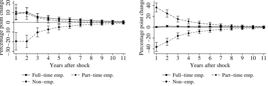
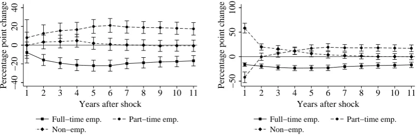
[image:24.595.88.516.396.533.2]t= 1). Vertical bars represent 95% confidence intervals. Confidence intervals were constructed from repeated evaluations of the effects of the policy interventions where each evaluation used a new parameter vector obtained by sampling from the asymptotic distribution of the MLEs.
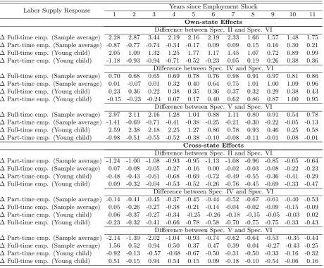
Figure 2(a) shows the average effect on the labor supply behavior of initially non-employed women of a temporary shock that moves non-employed women into full-time work. We see that this shock causes a significant increase in full-time work of 28.5 percentage points in the year immediately after the shock. The temporary shock continues to have a significant positive, but smaller, effect on full-time employment in subsequent years. This increase in full-time employment is balanced predominantly by a reduction in non-employment; the effect of the shock on part-time work is generally negative but is insignificant. Similarly, Figure 2(b) shows the average effect on the labor supply behavior of initially non-employed women of a temporary shock that moves non-employed women into part-time work. Such a shock causes a significant increase in part-time work, and a much smaller, yet significant, increase in full-time work, together balanced by a reduction in non-employment. Specifically, the one year own-state dependence effect for part-time employment is 33.3 percentage points, which is around 5 percentage points larger than the corresponding own-state dependence effect for full-time employment. Further, one year after a temporary shock that moves initially non-employed women into part-time work the rate of full-time employment is 2.7 percentage points higher than in the absence of any shocks, and this effect is significant at the 1.538% level. Due to the asymmetric nature of the cross-state dependencies and the higher own-state dependence in part-time employment as compared to full-time employment, a shock that increases part-time employment produces a larger reduction in non-employment than does a shock that increases full-time employment. This result highlights the value of our multinomial approach to modeling labor supply; a binary model of labor force participation would be uninformative about the relative merits of labor market policies that facilitate either full-time or part-time employment.
5.3 Heterogeneity in Labor Supply Dynamics after Child Birth
We use the parameter estimates for Specification VI to explore the extent of heterogeneity in labor supply dynamics following the birth of a child. As discussed in Section 5, Table 3 shows that there are significant amounts of variation in the effects of having a child aged under one year on a woman’s payoffs from both full-time and part-time work. Together with the significant state dependence effects documented above, heterogeneity in the effects of having a child aged under one year suggests that there may be persistent differences in labor supply behavior following the birth of a child.
Figure 3 shows the estimated effect a having a child on subsequent employment behavior for women at different points in the distribution of unobserved preferences for full-time and part-time work in the event that they have a child aged under one year. Figure 3(a) shows that for women who have a high unobserved preference for full-time work in the event that they have a child aged under one year, having a young child has very little immediate effect on labor supply behavior. As the child becomes older these women become more likely to work part-time and less likely to work full-time, as compared to if they had not had a child. Non-employment increases slightly 3-6 years following the birth of the child. Thus, we conclude that for women with a very strong preference for full-time work in the event that they have a child aged under one year, there is a substitution away from full-time work and towards part-time work, but no pronounced movement away from employment in general.
We see from Figure 3(b) that the picture is dramatically different for women who have a relatively low preference for full-time work in the event that they have a child aged under one year. For such women, the birth of a child is accompanied by a large and significant substitution away from both full-time and part-time work and into non-employment. For such women, two years after the shock the rate of part-time employment is higher than if the women had not had a child, however it takes 6 years before the rate of non-employment among women with a low preference of full-time work in the event that they have a child aged under one year is within two percentage points of the rate of non-employment among women with a high preference of full-time work in the event that they have a child aged under one year. Figures 3(c) and 3(d) illustrate the change in labor supply behavior over time caused by the birth of a child for women with high and low preferences for part-time work in the event that they have a child aged under one year. We see that the variation in employment responses according to the unobserved tastes for part-time employment in the event that the woman has a child aged under one year is very similar to the variation on employment responses according to tastes for full-time employment in the same circumstances. This latter result reflects the high correlation between the incremental unobserved components of preferences for full-time and part-time work that occur due to the presence of a child aged under one year.
5.4 Comparisons with More Restrictive Specifications