Novel Adaptive Evolutionary Computation Approaches
to the Dynamic Economic Load Dispatch Problems with
Non-Smooth Fuel Cost Function
Sunny Orike
Department of Computer Science Heriot-Watt University Edinburgh, United Kingdom
ABSTRACT
The paper presents novel approaches to solving the dynamic economic load dispatch (DELD) problem with valve-point loading effects. In dynamic environments, optimization problems change over time. They are also called time dependent or dynamic time-linkage problems, where decisions made at a given time may affect output obtained in a later time. It is therefore expected of algorithms solving dynamic optimization problems to both locate optimal solutions of the given problem and keep track of such solutions as they change with time. An investigation was made of three optimization methods in conjunction with three smart mutation variants, on benchmark problem cases involving 5 and 10 generating units, the major test cases in the literature with comparative results for other algorithms. The results suggest that the third approach which exploits the dynamic nature of the problem was capable of superior to the other two approaches. Comparisons with all approaches so far in the literature that have addressed these problems show that these evolutionary computation approaches are superior to other algorithms.
General Terms
Algorithm, Artificial Intelligence, Optimization, Electrical Power System, Performance, Simulation
Keywords
Economic Load Dispatch, Evolutionary Computation, Fitness Evaluation, Ramp-Rates, Valve-Point Effects
1.
INTRODUCTION
A great majority of problems in real-world applications are very complex and adaptive, as well as ways and methods used in solving them. The solutions are obtained by balancing several (and sometimes) conflicting multiple criteria in dynamic environments. Artificial intelligent techniques present powerful machine learning and nature-inspired approaches to investigate ways of solving problems in such dynamic environments which pose great challenges. This is the case of electrical power system optimization problems with multiple objectives, challenging constraints and dynamic demands. Here, there are constant changes affecting the power variables, various problem scenarios, with lots of operational constraints, resulting in the optimal solutions changing over time, and across dispatch periods.
The Economic Load Dispatch (ELD) problem is concerned with the determination of the optimal combination of electrical power output for generating units in power stations on a near-real time basis, and with respect to a predicted load
demand. The aim is to minimize the cost of producing power among those units (basically fuel cost), while obeying all operational constraints.
The Dynamic Economic Load Dispatch (DELD) problem extends the traditional, also called Static Economic Load Dispatch (SELD) problem. It exists in practical systems involving ramp-rate limits (which constrain the changes that can be made to the settings of an individual generator between periods), where operational decisions at a given hour will affect the decision at a later hour [1]. This is one of several optimization problems that need repeatedly to be solved in the electricity industry. Formulation of DELD addresses two major issues: (1) the changes caused by ramp-rate limits, which makes the power generation to be periodically adjusted to meet targeted demands; and (2) the dynamic costs involved in changing from one output level to another [2]. This makes it a more applicable formulation of the economic load dispatch problem, but also a more difficult and complex optimization problem. Until now, the DELD has been treated as a series of unconnected static problems.
estimate a probability distribution from population of solutions, and sample it to generate the next population.
EC remains an active area of research in the entire field of computational intelligence. Other recent approaches are: Expert System, Tabu Search, Shuffled Frog Leaping Algorithm and Artificial Immune System [5]. Expert System, first proposed by Feigenbaum et al in the early 1970s [6], is a knowledge-based method, which uses the knowledge and interface procedure to solve problems that are difficult enough to require human expertise for their solution. Tabu Search is an iterative gradient-descent search algorithm with memory and response exploration [7]. The memory stores a number of previously visited states, along with a number of unwanted states in a Tabu list. Shuffled Frog Leaping Algorithm (SFLA), proposed by Eusuff and Lansey in 2003 [8], involves a set of frogs that co-operate with each other to achieve a unified behavior for the whole system. Artificial Immune System, inspired by the works of Farmer, Packard and Perelson in 1986 [9], is a class of computationally intelligent systems based on the principles and processes of the immune system. It combines the characteristics of learning and memory of the system to solve a problem.
This paper is organized as follows: Section 2 reviews previous DELD solution approaches in the literature, Section 3 shows the problem formulation; Section 4 describes the proposed optimization algorithm; Section 5 details the experimental design, results and discussions; while Section 6 concludes the findings of the work.
2.
REVIEW OF PREVIOUS DELD
OPTIMIZATION APPROACHES
All The development of DELD formulations and approaches is a dynamic research area, due to the dynamic nature of power systems and large variations of load demands. A number of methods have been adopted in solving DELD problems with non-smooth and non-convex cost functions. A major common difficulty with all the methods is choosing control parameters. In [10], General Algebraic Modelling System (GAMS) was proposed for different cases of DELD problems involving six generating units with a consideration of cost, losses and emissions. GAMS consist of a collection of statements in high-level language used to represent problem models. It performs the required data transformation to instantiate the model, which could be applied to linear, non-linear as well as mixed-integer optimization problems. The various components of the system are: sets, data, variables, equations, model/solution, and output statements. The solution approach is analytic in nature with good computational efficiency, high accuracy and environment friendly, but it will be very cumbersome for solving large, complex and adaptive DELD systems. Maclaurin Series-Based Lagrangian Method was proposed in [2], where the sinusoidal component of the cost function is represented by a series of Maclaurin approximation, solved using Lagrangian method to realise an optimal or near optimal solution in a single run. The approach is simple and easy to implement, with a fast convergence rate, low computational time demands, and produces a unique solution. However, it is mainly applicable to relatively simple functions. A simple and direct Sequential Approach with Matrix Framework was developed in [11]. The aim is to determine optimal generation dispatches across the entire periods in a single execution. While the effectiveness of the approach was validated in some benchmark cases involving fewer test systems, for large power systems, it suffers from the curse of dimensionality due to the matrix size and coupled with the sequentiality of the
algorithm. Evolutionary and other stochastic methods such as: Genetic Algorithm (GA) [12], Fuzzy Logic (FL) [13], Artificial Neural Network (ANN) [7], Particle Swarm Optimization (PSO) [4], Differential Evolution [14], Simulated Annealing (SA) [15], their hybrids and variants including: Hopfield Neural Network/Quadratic Programming [16], Harmony Search Algorithm [17], Evolutionary Programming/Sequential Quadratic Programming [18], Fuzzy Logic/Simulated Annealing [19], etc, have attracted great interest in the recent past for realising optimal solutions, and applied to solve DELD problems. These algorithms are population-based search methods, with random control parameters, and use probabilistic rules to update the positions of their potential solutions in the search space. But in most often times, there is no guarantee of finding global optimum solutions, only feasible solutions are realised within a reasonable time frame. However, where the number of the search variables and parameters are large and highly correlated, realising global optimal solutions becomes a problem due to the large dimensionality of the dynamic dispatch. In [12], a calculus of variations and GA were jointly applied to optimize the DELD problem, with the GA focussing on penalty weighting parameters. However, a problem involving only 3 generating units was considered and they were not sure of its applicability to larger systems. Unless used as a hybrid tool with other approaches, the application of Fuzzy Logic to active power generation is very limited. For complex problems ANNs need to have many inputs and/or several layers of inputs; with consequently many parameters, much time is required for training, and good results are far from guaranteed. Although PSO has the ability of quick convergence through exploration, but it is very slow in exploitation, and when stuck, it encounters a problem while escaping from local optima. DE converges too quickly, and may not be a good approach for large scale optimization tasks. Setting of control parameters using SA is a very cumbersome task, leading to slow execution speed. In this paper, an investigation is made of novel adaptive algorithms involving three optimization approaches in conjunction with three variants of a smart mutation operator on bench mark dynamic problems with valve-point loading effects.
3.
DELD FORMULATION
The main objective of the DELD is to simultaneously minimize the generation cost and meet the consumers’ load demand over a given period of time while satisfying three major constraints: load balance, generation limit and ramp-rates constraints. For non-smooth cost function with valve-point loading effects, the objective function is represented as the sum of the smooth quadratic function and the absolute value of the sinusoidal function (1):
T t N i t i i i i t i i t i i iT a bPg cPg eSin f Pg Pg
F Min 1 1 , min 2 , , ( ( )) (1)
Subject to the generation limit and power balance constraints of (2) to (4):
max , min i t i
i
Pg
Pg
Pg
(2)
0 , , 1 ,
Dt Lt
N i
t
i P P
Pg
(3)
00
1 1 1
, 0 ,
,
, Pg B Pg B Pg B
P N i N j N i t i i t j ij t i t
L
Considering the ramp-rate limit constraint, there are three possible cases in actual operation of the generating units: steady state condition, increasing generation and decreasing generation conditions, as shown in (5) to (7).
1 ,
,t it
i Pg
Pg (5)
i t i t
i Pg UR
Pg, ,1
(6)
i t i t
i Pg DR
Pg,1 ,
(7)
Therefore the constraint of (2) due to the ramp-rate limits of (6) and (7) is modified as:
) ,
min( )
,
max(Pgimin,t Pgi,t1DRi Pi,t Pgimax,t Pgi,ttURi (8)
Where:
FT =Total operating cost over the whole dispatch period;
T = Number of time periods; N = Number of generating units; ai, bi, ci = Cost coefficients of i
th
unit with quadratic function; ei, fi = Cost coefficients of ith unit with sinusoidal function;
Pgi,t = Power output of i th
unit;
Pgi, t-1 = Power generation of ith unit at the previous period;
PD,t = Total power demand at period, t;
PL,t = Power losses at period, t;
Pgimin = Lower limit of the ith unit;
Pgimax = Upper limit of the ith unit;
URi = Ramp-up limit of unit i,
DRi = Ramp-down limit of unit i.
4.
OPTIMIZATION ALGORITHM
An investigation is made of three dynamic optimization approaches (D1, D2 and D3) in conjunction with three smart evolutionary algorithms (SEA1, SEA2 and SEA3) from the three variants of smart mutation operators developed in a previous work of [20], to solve the DELD problem with valve-point effects and ramp-rate constraints for a 24-hour dispatch period. Assuming there are N generators and T dispatch periods, the control variables are represented by an array with dimension N x T elements, and output of generator i at time t is given by Pgi,t; ranging from Pg11 to PgNT:
)] (
) [(
,t 11, 21, 31, N1 1T, 2T, NT
i Pg Pg Pg Pg Pg Pg Pg
Pg (9)
D1 is a baseline dynamic optimization method that solves the dynamic form of the problem in sequence of static problems; D2 solves the static problems together, treated as a single multi-part problem with suitably adjusted constraints; while D3 extends D2, with the final population of previous periods being used to initialise the populations of subsequent periods. SEA1 uses tournament selection based on the penalty values to decide which gene to mutate; SEA2 introduces a mutation probability, whereby a smart mutation is done when the probability is met, otherwise, a standard random mutation is done; SEA3 extends SEA2, but the value of the mutation probability starts at 0, and gradually moves to 1 in a linear fashion towards the probability is met, the maximum number of generations.
Starting with initial feasible solution vectors of (9), the following is the procedural description of the flow of work towards the realization of the solution to the DELD problem.
i. Read system data, dispatch period, and predicted load demand for each period.
ii. Initialise randomly at the first period, the population of chromosome within the generating units’ range, according to the specifications of D1, D2 and D3. iii. Uniform gene distribution ensures that the generators’
outputs are within the legal minimum and maximum limits defined in (10), through the following rules:
min min
max
,t * ()*( i i ) i
i rand Pg Pg Pg
Pg
(10)
Where: α is a scaling factor (user-defined small positive number less than one).
iv. With additional dynamic constraints involved (load balance and ramp rate limits) across the dispatch periods, processing constraints violation becomes a harder task. There exists also a complexity in realising an optimum solution in this formulation due to the presence of valve-point loading effects, which creates additional ruggedness in the cost curve and is likely to increase the density of local optima.
v. In a given dispatch period, the population of chromosomes contains feasible genes (outputs for each generating unit) which must be within the minimum and maximum generation limits according to (10). Checks are made to ensure that violations in power balance and ramp-rate limits constraints are handled. Violation of either or both of them constitutes the penalty in this case.
vi. Compute costs of individual genes using the objective function of (1).
vii. The genes with the highest cost, including those that violate load balance and/or ramp-rates constraints are subject of the smart mutation, see [20] for details. viii. The penalties augment the objective function to form
the generalised fitness function of equation (4.15), used in a similar problem case of [101, 108].
2 1 1 lim , 2 1 1 , , , 1 1 , min 2 , , ( ( ))
T t N i rr t i T t N i t L t D t i T t N i t i i i i t i i t i i i T Pg Pg P P Pg Pg Pg f Sin e Pg c Pg b a F (11)Where: μ and β are penalty terms which reflect the violation of the power balance and ramp-rates constraints respectively, assigning a high cost of penalty to affected ones far from the feasible region [14], and the outputs of the generating units due to the dynamic ramp-rate limits are defined by:
otherwise Pg UR Pg Pg UR Pg DR Pg Pg DR Pg Pg t i i t i it i t i i t i it i t i rr , , , , , , 1 , 1 , 1 , 1 , lim (12)
ix. Output the best compromising solution vector for each of the dispatch periods:
)] (
) [(
,t 11, 21, 31, N1 1T, 2T, NT
i Pg Pg Pg Pg Pg Pg Pg
5.
EXPERIMENTAL DESIGN AND
ANALYSIS OF RESULTS
The performances of the dynamic optimization approaches D1, D2 and D3 in conjunction with three smart evolutionary algorithms (SEA1, SEA2 and SEA3) were tested in two different experimental cases involving 5 and 10 units systems, the major test cases in the literature for which there are comparative results for other algorithms.
5.1 Five (5) Generating Units
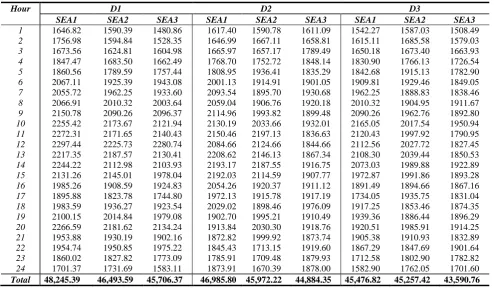
[image:4.595.52.547.197.486.2]The generators’ data, loss coefficients matrix and load demand in each hour were taken from [2, 14]. The dispatch period is an arbitrary 24 hours and losses were considered. Simulation of the algorithm was made for 30 runs, with the hourly costs for SEA1, SEA2 and SEA3 in each of D1, D2 and D3 given in Table I, while Table II compares the results with other approaches in the literature using the same set of data.
Table I. Hourly costs of the 9 dynamic approaches, averaged over 30 runs on the 5-unit problem
Hour D1 D2 D3
SEA1 SEA2 SEA3 SEA1 SEA2 SEA3 SEA1 SEA2 SEA3
1 1646.82 1590.39 1480.86 1617.40 1590.78 1611.09 1542.27 1587.03 1508.49 2 1756.98 1594.84 1528.35 1646.99 1667.11 1658.81 1615.11 1685.58 1579.03 3 1673.56 1624.81 1604.98 1665.97 1657.17 1789.49 1650.18 1673.40 1663.93 4 1847.47 1683.50 1662.49 1768.70 1752.72 1848.14 1830.90 1766.13 1726.54 5 1860.56 1789.59 1757.44 1808.95 1936.41 1835.29 1842.68 1915.13 1782.90 6 2067.11 1925.39 1943.08 2001.13 1914.91 1901.05 1909.81 1929.46 1849.05 7 2055.72 1962.25 1933.60 2093.54 1895.70 1930.68 1962.25 1888.83 1838.46 8 2066.91 2010.32 2003.64 2059.04 1906.76 1920.18 2010.32 1904.95 1911.67 9 2150.78 2090.26 2096.37 2114.96 1993.82 1899.48 2090.26 1962.76 1892.80 10 2255.42 2173.67 2121.94 2130.19 2033.66 1932.01 2165.05 2017.54 1950.94 11 2272.31 2171.65 2140.43 2150.46 2197.13 1836.63 2120.43 1997.92 1790.95 12 2297.44 2225.73 2280.74 2084.66 2124.66 1844.66 2112.56 2027.72 1827.45 13 2217.35 2187.57 2130.41 2208.62 2146.13 1867.34 2108.30 2039.44 1850.53 14 2244.22 2112.98 2103.93 2193.17 2187.55 1916.75 2073.03 1989.88 1922.89 15 2131.26 2145.01 1978.04 2192.03 2114.59 1907.77 1972.87 1991.86 1893.28 16 1985.26 1908.59 1924.83 2054.26 1920.37 1911.12 1891.49 1894.66 1867.16 17 1895.88 1823.78 1744.80 1972.13 1915.78 1917.19 1734.05 1935.75 1831.04 18 1983.59 1936.27 1923.54 2029.02 1898.46 1976.09 1917.25 1853.46 1874.35 19 2100.15 2014.84 1979.08 1902.70 1995.21 1910.49 1939.36 1886.44 1896.29 20 2266.59 2181.62 2134.24 1913.84 2030.30 1918.76 1920.51 1985.91 1914.25 21 1953.88 1930.19 1902.16 1872.82 1999.92 1873.74 1905.38 1910.93 1832.89 22 1954.74 1950.85 1975.22 1845.43 1713.15 1919.60 1867.29 1847.69 1901.64 23 1860.02 1827.82 1773.09 1785.91 1709.48 1879.93 1712.58 1802.90 1782.82 24 1701.37 1731.69 1583.11 1873.91 1670.39 1878.00 1582.90 1762.05 1701.60
Total 48,245.39 46,493.59 45,706.37 46,985.80 45,972.22 44,884.35 45,476.82 45,257.42 43,590.76
Table II. Summary of costs of the 9 dynamic approaches, averaged over 30 runs and comparison with other approaches on the 5-unit problem
Approach Min Cost ($/hr) Av Cost ($/hr) Max Cost ($/hr)
PSO [2] 50,124.00 - -
PSO [1] 49,970.43 50216.59 51803.30
MSL [2] 49,216.81 - -
SA [15] 47,356.00 - -
DE [17] 43,213.00 43,813.00 44,247.00
HHS[1] 43,154.86 - -
D1_SEA1 46,985.74 48,245.39 49,417.14
D1_SEA2 45,414.51 46,493.59 49,711.25
D1_SEA3 44,810.20 45,706.37 46,655.38
D2_SEA1 45,680.25 46,985.80 48,104.08
D2_SEA2 42,125.08 45,972.22 47,379.97
D2_SEA3 38,638.89 46,884.35 48,437.36
D3_SEA1 44,325.67 45,476.82 46,451.82
D3_SEA2 41,704.25 45,257.42 48,280.88
[image:4.595.146.450.538.712.2]Figure 1: Variation of costs of the best two approaches (D2_SEA3 and D3_SEA3) on the 5-unit problem
[image:5.595.64.268.74.237.2]for this problem, with the former having the lowest minimum cost and the latter having the lowest average cost, over 30 runs among the 9 approaches. To further explore the differences between the two approaches, a plot of the variation of their generation costs across the 24 hours dispatch period was made, as shown in Figure 1 (averaged over 30 runs). From the curve, it is clear that D3_SEA3 outperforms D2_SEA3. Figure 2 is a load curve distribution comparing the best and worst approaches (D3_SEA3 and D1_SEA1) respectively, with the load demand across the entire dispatch. Being a smaller problem case, all the 9 dynamic approaches performed relatively well, confirming the performance efficiency of the approaches. Table III shows typical (best) resources scheduling using the best approach.
Figure 2: Load curve comparing the best approach (D3_SEA3), worst approach (D1_SEA1), with load
demand on the 5-unit problem
5.2
Ten (10) Generating Units
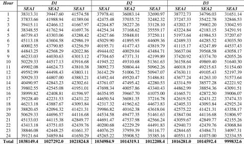
The generators’ data, loss coefficients matrix and load demand in each hour were taken from [2, 14]. The dispatch period is an arbitrary 24 hours and transmission losses were ignored for ease of comparison of results with those of other approaches reported in literature. Table IV shows the hourly costs (averaged over 30 runs) for SEA1, SEA2 and SEA3 in each of D1, D2 and D3 throughout the entire dispatch period, while Table V compares the results with other approaches in the literature using the same set of data. Table V reveals comparatively lower costs from D1_SEA3, D3_SEA2 and D3_SEA3 out of the 9 dynamic approaches for this problem, in terms of total minimum and average costs. Figure 3 shows the variation of their average total costs across the 24 hours dispatch period (over 30 runs), while Figure 4 compares the load curve distribution of the best and worst approaches across the entire dispatch period. Again, from the two figures, D3_SEA3 seems to be the best optimizer for this problem, with lower cost (Figure 3), and its load trend (Figure 4). Overall, the results indicate that D3_SEA3 is generally the choice to be recommended. Table VI shows a best resources scheduling using the best approach.
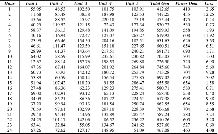
Table III. Typical resources scheduling in a single run of the best DELD approach on the 5-unit problem
Hour Unit 1 Unit 2 Unit 3 Unit 4 Unit 5 Total Gen Power Dem Loss
1 55.95 48.53 102.50 101.75 103.91 412.65 410 2.65
2 11.68 85.48 38.58 187.98 123.53 447.25 435 12.25
3 45.66 88.52 45.97 220.10 75.19 475.44 475 0.44
4 40.29 119.52 121.15 72.43 177.34 530.73 530 0.73
5 58.37 36.13 129.48 141.09 194.85 559.93 558 1.93
6 40.16 116.94 72.47 127.07 263.27 619.92 608 11.92
7 23.99 66.46 154.50 204.16 182.51 631.63 626 5.63
8 46.61 111.47 123.59 151.18 227.65 660.51 654 6.51
9 28.99 61.37 143.64 217.51 240.21 691.71 690 1.71
10 64.02 58.59 115.99 235.61 230.82 705.03 704 1.03
11 12.67 88.14 157.76 198.53 269.80 726.90 720 6.90
12 47.36 67.41 164.07 201.92 264.84 745.60 740 5.60
13 60.73 75.93 142.12 180.72 253.79 713.28 704 9.28
14 53.89 60.59 150.14 156.54 275.85 697.02 690 7.02
15 51.94 107.42 118.20 91.55 286.47 655.58 654 1.58
16 27.48 86.36 62.23 129.23 275.41 580.71 580 0.71
17 69.00 102.91 93.12 65.13 228.24 558.40 558 0.40
18 34.09 85.21 86.36 187.22 224.51 617.38 608 9.38
19 37.20 99.94 93.13 181.54 250.74 662.55 654 8.55
20 70.59 97.61 102.99 207.10 228.39 706.68 704 2.68
21 29.48 94.44 44.96 132.89 285.47 587.24 580 7.24
22 24.29 101.17 142.06 86.52 256.22 610.26 605 5.20
23 63.41 32.84 55.05 134.67 241.62 527.60 527 0.60
24 67.26 72.62 127.17 148.95 51.09 467.08 463 4.08
0 500 1000 1500 2000
0 4 8 12 16 20 24
Period (Hour)
A
v
g
T
o
ta
l
C
o
st
s
($
)
D2_SEA3 D3_SEA3
400 500 600 700 800
0 4 8 12 16 20 24
Period (Hours)
P
ow
e
r
O
u
tp
u
t (M
W)
[image:5.595.109.489.536.770.2]Table IV. Hourly costs of the 9 dynamic approaches, averaged over 30 runs on the 10-unit problem
Table V. Summary of results, over 30 runs and comparison with other approaches on the 10-unit problem
Approach Minimum
Cost ($/hr)
Average Cost ($/hr)
Maximum Cost ($/hr) PSO [1] 1,052,655.81 1,055,963.30 1,046,633.42
SQP [17] 1.051,163.00 - -
EP [17] 1,048,638.00 - -
EP-SQP [18] 1,031,746.00 1,035,748.00 -
DE [14] 1,019,786.00 - -
HHS [17] 1,019,019.11 - -
D1_SEA 1 1,027,664.37 1,038,149.43 1,046,674.90 D1_SEA 2 1,003,166.34 1,027,291.99 1,217,239.92 D1_SEA 3 894,893.10 1,021,824.75 1,234,955.97 D2_SEA 1 930,464.83 1,034,984.93 1,142,581.07 D2_SEA 2 983,428.21 1,014,319.09 1,055,054.96 D2_SEA 3 996,122.31 1,012,208.44 1,030,564.23 D3_SEA 1 959,565.27 1,016,280.95 1,090,724.60 D3_SEA 2 887,541.23 1,014,592.37 1,088,462.06 D3_SEA 3 907,838.55 999,832.63 1,021,407.08
Hour D1 D2 D3
SEA1 SEA2 SEA3 SEA1 SEA2 SEA3 SEA1 SEA2 SEA3
Figure 3: Variation of costs of the best 3 dynamic
[image:7.595.322.541.73.245.2]approaches, in the entire dispatch on the 10-unit problem Figure 4 Load curve comparing the best and worst approaches, with load demand on the 10-unit problem
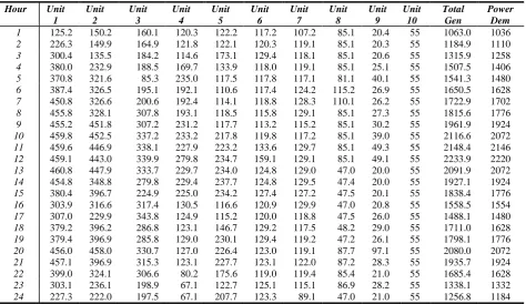
Table VI. Best resources scheduling in a single run of the best DELD approach on the 10-unit problem
Hour Unit
1
Unit 2
Unit 3
Unit 4
Unit 5
Unit 6
Unit 7
Unit 8
Unit 9
Unit 10
Total Gen
Power Dem
1 125.2 150.2 160.1 120.3 122.2 117.2 107.2 85.1 20.4 55 1063.0 1036 2 226.3 149.9 164.9 121.8 122.1 120.3 119.1 85.1 20.3 55 1184.9 1110 3 300.4 135.5 184.2 114.6 173.1 129.4 118.1 85.1 20.6 55 1315.9 1258 4 380.0 232.9 188.5 169.7 133.9 118.0 119.1 85.1 25.1 55 1507.5 1406 5 370.8 321.6 85.3 235.0 117.5 117.8 117.1 81.1 40.1 55 1541.3 1480 6 387.4 326.5 195.1 192.1 110.6 117.4 124.2 115.2 26.9 55 1650.5 1628 7 450.8 326.6 200.6 192.4 114.1 118.8 128.3 110.1 26.2 55 1722.9 1702 8 455.8 328.1 307.8 193.1 118.5 115.8 129.1 85.1 27.3 55 1815.6 1776 9 455.2 451.8 307.2 231.2 117.7 113.2 115.2 85.1 30.2 55 1961.9 1924 10 459.8 452.5 337.2 233.2 217.8 119.8 117.2 85.1 39.0 55 2116.6 2072 11 459.6 446.9 338.1 227.9 223.2 133.6 129.7 85.1 49.3 55 2148.4 2146 12 459.1 443.0 339.9 279.8 234.7 159.1 129.1 85.1 49.1 55 2233.9 2220 13 460.8 447.9 333.7 229.7 234.0 124.8 129.0 47.0 20.0 55 2091.9 2072 14 454.8 348.8 279.8 229.4 237.7 124.8 129.5 47.4 20.0 55 1927.1 1924 15 380.4 396.7 224.9 225.0 234.2 127.4 127.2 47.5 20.1 55 1838.4 1776 16 303.9 316.6 317.4 130.5 116.6 120.9 129.9 47.0 20.8 55 1558.5 1554 17 307.0 229.9 343.8 124.9 115.2 120.0 118.8 47.5 26.0 55 1488.1 1480 18 379.2 396.2 286.8 123.1 146.7 129.2 117.5 48.2 29.0 55 1711.0 1628 19 379.4 396.9 285.8 129.0 230.1 129.4 119.2 47.2 26.1 55 1798.1 1776 20 456.0 458.0 330.7 127.0 226.4 123.0 119.1 87.7 97.1 55 2080.0 2072 21 457.1 396.9 315.3 123.1 227.7 123.1 122.0 87.2 28.3 55 1935.7 1924 22 399.0 324.1 306.6 80.2 175.6 119.0 119.4 85.4 21.0 55 1685.4 1628 23 303.1 236.1 198.9 67.1 122.7 125.1 115.1 86.9 28.2 55 1338.1 1332 24 227.3 222.0 197.5 67.1 207.7 123.3 89.1 47.0 21.0 55 1256.8 1184
6.
CONCLUSION
The paper presented novel approaches to solving DELD problem with non-smooth objective cost functions with valve- point loadings effect, consisting of quadratic function and the absolute value of the sinusoidal function. Guided by a smart evolutionary algorithm (which combines a standard GA with smart mutation operator that focuses mutation on genes that contribute mostly to cost and penalty violations), and approaches that provided superior results on in the case of static ELD problems, an attempt was made to adapt these for the dynamic context. In the experimental design, an investigation was made of three optimization methods in conjunction with three smart mutation variants, on benchmark cases involving 5 and 10 generating units, the major test cases
in the literature with comparative results for other algorithms. They are: (1) treating the DELD simply as a series of static problems, (2) treating them as a single many-parameter problem, and (3) a basic dynamic optimization approach, in which the final population of one part of the DELD became the initial population for the next. From the results, the performance of the third approach (D3), which was superior to the other two approaches (D1 and D2). Comparisons with all approaches so far in the literature that have addressed these problems show that these EC-based approaches, especially D3_SEA3 is superior to other algorithms (see Tables II and V). In both test cases, the best average and minimum costs are better than those of the published approaches whenever the comparative figure is obtainable.
0 10000 20000 30000 40000 50000
0 4 8 12 16 20 24
Period (Hours)
A
vg
To
tal
C
os
t ($
)
D1_SEA3 D3_SEA2 D3_SEA3
800 1200 1600 2000 2400
0 4 8 12 16 20 24
Period ( in Hour)
P
ow
er
O
u
tp
u
t (M
W)
[image:7.595.62.537.324.598.2]The contributions in this paper are partly in the area of applied computer science and partly in regard to the specific application area (electrical power system optimization). Areas of future work similarly align with these two areas of contribution. The results of this paper showed that the third optimization approach seems promising in this application. However, there are so many possibilities that could be tried here, such as using elitism, i.e., by keeping the best percentage of the population unchanged, and randomly generating the rest, or keeping the best population unchanged, and generate the rest through mutations applied to these best populations.
7.
REFERENCES
[1] G. Sreenivasan, C. H. Saibabu and S. Sivanagaraju, “Solution of Dynamic Economic Load Dispatch Problem with Valve Point Loading Effects and Ramp Rate Limits using PSO”, International Journal of Electrical and Computer Engineering, vol. 1, no. 1, pp. 59 – 70, 2011.
[2] S. Hemamalini and S. P. Simon, “Dynamic Economic Dispatch Problem with Valve Point Effects using Maclaurin Series Based Lagrangian Method”, International Journal of Computer Applications (0975-8887), vol. 1, no. 17, pp. 71 – 77, 2010.
[3] Poole, D., Mackworth, A. and Goebel, R. 1999. Computational Intelligence, a Logical Approach, Oxford University Press.
[4] Goldberg, D. E. 1989. Genetic Algorithms in Search, Optimization and Machine Learning. Addison Wesley.
[5] R. C. Bansal, “Optimization Methods for Electrical Power Systems: An Overview”, Journal for Emerging Electric Power Systems, vol. 2, no. 1, pp. 1 – 23, 2005.
[6] D. Saxena, S. N. Singh and K. S. Verma, “Application of Computational Intelligence in Emerging Power Systems”, International Journal of Engineering, Science and Technology, vol. 2, no. 3, pp 1 – 7, 2010.
[7] R. C. Bansal, “Literature Survey on Expert System Applications to Power Systems”, International Journal Engineering Intelligent Systems, vol. 11, no. 3, pp.103 – 112, 2003.
[8] M. Eusuff and K. Lansey, “Optimization of Water Distribution Network Design using the Shuffled Frog Leaping Algorithm,” Journal of Water Resources Planning and Management, vol. 129, no. 3, pp. 210 –225, 2003.
[9] J. D. Farmer, N. Packard and A. Perelson, “The Immune System, Adaptation and Machine Learning”, Physica D, vol. 2, pp. 187–204, 1986.
[10]D. Bisen and H. M. Dubey, “Dynamic Economic Load Dispatch with Emission and Loss using GAMS”, International Journal of Engineering Research and Technology, vol. 1, no. 3, pp. 1 – 7, 2012.
[11]S. Ganesan and S. Subramanian, “Dynamic Economic Dispatch Based on Simple Algorithm”, International Journal of Computer and Electrical Engineering, vol. 3, no. 2, pp. 1793 – 8163, 2011.
[12]K. Asano, M. Nakatsuka and T. Kumano, “Calculus of Variation and Genetic Algorithm considering Ramp Rate”. In Proceedings of 15th International Conference on Intelligent System Applications to Power Systems, Curitiba, 2009.
[13]P. Attaviriyanupap, H. Kita, E. Tanaka and J. Hasegawa, “A Fuzzy-Optimization Approach to Dynamic Economic Dispatch Considering Uncertainties”, IEEE Transactions of Power Systems, vol. 19, no. 3, pp. 1299 – 1307, 2004.
[14]R. Balamurugan and S. Subramanian, “Differential Evolution-based Dynamic Economic Dispatch of Generating Units with Valve-point Effects”, Journal of Electrical Power Components and Systems, vol. 36, no. 8, pp. 828 – 843, 2008.
[15]C. K. Panigrahi, P. K. Chattopadhyay, R. N. Chakrabarti, M. Basu, “Simulated Annealing Technique for Dynamic Economic Dispatch”, Journal of Electrical Power Components Systems Research, vol. 34, no. 5, pp. 577 – 586, 2006.
[16]S. F. Mekhamer, A. Y. Abdelaziz, M. Z. Kamh and M. A. L. Badr, “Dynamic Economic Dispatch using a Hybrid Hopfield Neural Network/Quadratic Programming Based Technique”, Journal of Electrical Power Components and Systems, vol. 37, no. 3, pp. 253 – 264, 2009.
[17]V. R. Pandi and B. K. Panigrahi, “Dynamic Economic Load Dispatch using Hybrid Swarm Intelligence Based Harmony Search Algorithm,” Journal of Expert Systems with Applications, vol. 38, pp. 8509 – 8514, 2011.
[18]P. Attaviriyanupap H. Kita, E. Tanaka and J. Hasegawa, “A Hybrid EP and SQP for Dynamic Economic Dispatch with Non-Smooth Fuel Cost Function”, IEEE Transactions on Power Systems, vol. 17, no. 2, pp. 411 – 416, 2002.
[19]M. Basu, “An Interactive Fuzzy Satisfying-based Simulated Annealing Technique for Economic Emission Load Dispatch with Non-Smooth Fuel Cost and Emission Level Functions”, Electrical Power Components and Systems, vol. 32, no. 2, pp. 163 – 173, 2010.