http://dx.doi.org/10.4236/gep.2014.23014
Some Mass Migration Underground Found
in Beijing Area
Zheng Xin Li1,2, Jin Song Ping1,2, Yong Zhang Yang1,2, Alexander Gusev1
1Key Laboratory of Lunar and Deep Space, National Astronomical Observatories, Chinese Academy of Sciences,
Beijing, China
2Center of Astrodynamic Research, Shanghai Astronomical Observatory, Chinese Academy of Sciences,
Shanghai, China
Email: [email protected], [email protected]
Received April 2014
Abstract
The relationship between the change of a local gravity field and the mass migration underground is discussed by means of using a point-source disturbed body as a substitute for the mass migra-tion underground. Some significant local gravity field changes in Beijing area have been found, from which the three parameters of the disturbed bodies, location, depth and mass, have been de-rived successfully from the observations of a gravimetric network. In order to determine the depth of a body, a new approach is suggested in which the gravity change difference is used in-stead of the gravity change itself. The mass of a disturbing body has been estimated properly. As-tronomical PZT is suggested for this kind of survey. The results provide us a picture of the under-ground mass migration with which the gravity changes on the under-ground surface may be interpreted in a better way. This additional information may be useful in seismological studies.
Keywords
Component, Underground Mass Migration, Gravity Field, Earthquake, PZT
1. Introduction
Gravity change and earthquake (Barnes, 1966), or furthermore, the relationship among gravity change, under-ground mass migration and earthquake (Chen et al., 1979), is an interesting but unsolved problem for many years (Chen et al., 2002). The China Beijing-Tianjin-Tangshan-Zhangjiakou (BTTZ) gravimetric network was established in 1980’s (Chen et al., 2002), and its observational data have been used heavily in studying the problem (Gu et al., 1998; Kuo et al., 1993; Kuo et al., 1999; Jia et al., 1998; Li et al., 2001; Jia et al., 2006). Due to the incompleteness of the network, which is based on the observations of relative gravimeter, the image of the relationship among the gravity change, underground mass migration and earthquake is still not clear (Chen et al., 2002).
which the related UDBs are studied. The three parameters of a UDB (location, depth and mass) are derived by a new approach, including a special order to calculate them. First measure the location, second the depth, third the mass; and then use the difference of gravity change in depth calculation instead of using the gravity change itself; and the mass estimation is the last step. It is hoping that the results will be helpful in understanding the problems mentioned above, as well as the related studies in seismology.
2. Formulae
Assume a mass migration, limited both in depth and size, has taken place underground during a time period and makes the local gravity field change. We use a point-source disturbed body underground, which is able to make the same gravity field change, to describe it, and try to determine its three parameters: location, depth (H) and mass (M).
An observer on ground, whose horizontal distance is D to the body site, will thus observe a gravity vector change with module of Δg = GM/S2 (G-gravity constant), pointing to the body with distance of S (S = (D2 +
H2)1/2). A gravimeter observes the vertical element while the horizontal one can be deduced from the observa-tion of an astronomical instrument. The vector is expressed by the following two elements in a vertical plane (Zhang et al., 2002):
The vertical element is read as:
(
)
3gv g H S/ GMH S/
∆ = ∆ = (1)
The horizontal element, or the deflection of the vertical (DOV) is read as:
(
)
3gh g D S/ GMD S/
∆ = ∆ = (2)
The two unknowns of the underground disturbed body, the H and M, may be determined by the Δgv, as well
as the Δgh, observed at separate places to which the distances Ds are known.
Instead of using the Δgv, or Δgh, itself directly, the ratio of them at two sites, No.1 and 2, may be used as an assumed “observation” Kv, or Kh, and use one of the following equations to calculate the unknown H:
(
)
3(
(
) (
)
)
3/ 22 2 2 2
(1) (2) 2 1 2 1
gv gv S /S D H / D H
= ∆ ∆ = = + +
Kv (3)
(
) (
)
3(
)
(
2 2)
2 2 3/ 2(1) (2) 1 2 2 1 1 2 2 1
gh gh D /D S /S D /D ( D H / (D H ))
= ∆ ∆ = × = × + +
Kh (4)
in which, D1 and D2 are the known horizontal distances of the two observational sites. The differential of Δgv may also be used in such a determination, which is derived as:
(
)
(
5)
(
2)
d / dD ∆gv = −3 GMDH S/ = −3 H S/ × ∆gh (5)
thus we have:
(
)
gh d / dD gv
∆ =Khv× ∆ (6) in which
( )
(
2)
- 1 / 3 S /H= ×
Khv (7)
The ratio Kdv of two Δgv differentials can be expressed as the following:
(
)
(
)
(
) (
)
51 2 2 1 (1) (2)
d / dD gv / d / dD gv D /D S /S
= ∆ ∆ = ×
Kdv (8)
(
)
(
)
(
)
(
(
) (
)
)
5/ 22 2 2 2
1 2 2 1
(1) (2)
d / dD gv / d / dD gv D /D D H / D H
= ∆ ∆ = × + +
Kdv (9)
from which the depth of the disturbed body (H) may also be calculated.
Having the H, the mass of the disturbed body M may then be calculated by the following equation but in term of its ratio to Earth mass (ME):
from the Δgv
(
) (
) (
)
20
/ gv / g / /
from the Δgh
(
) (
) (
)
20
/ gh / g / /
M ME = ∆ × S D ∗ S RE (11) in which RE is the Earth radius (6371 km), g0 is the gravity on ground (use g0 = 981 Gal), and ME = 5.9742 × 1024 kg.
In Figure 1, the maximum observed Δgv, while observer is just upside the body, is used as the unit (100%) in
showing the Δgv, Δgh and d/dD(Δgv); their horizontal distance to the body site is count by unit of H. It can be seen that Δgh has a peak (38%) at the distance of 0.7Hand becomes the same as the Δgv (36%) at distance of H, then decreasing to less than 5% when D > 5H. If we use 5% as a standard of gathering observations with enough sense, we may see that the area of meaningful Δgh observations (4.3H) is larger than that of the Δgv (2.5H).
Khv (see Equation (7)) is also shown in Figure 1, but with a different scale, which varies within −8.66 to −0.33 while −5 < D < 5.
3. BTTZ Gravimetric Network and the Local Gravity Field Change
The BTTZ gravimetric network (Figure 2) is located in north China and has more than hundred network points, 2 - 4 batch repeated observations per year, high precision of observations, and its continuation since 1987 (Chen et al., 2002; Li et al., 2005), are making it an appropriate place to study the problem of underground mass mi-gration.
LaCoste & Romberg G model gravimeter are used in relative measurement between two neighboring network points with precision of about ±7 ~ 10 micro Gal (Li et al., 2001). In addition, absolute gravimeter has also been performed from time to time at some network points in order to connect the observations of different batches together (Jia et al., 2006). Processing a batch observations, which have been completed in a short time, by the National Standard (Liu et al., 1991) and takes their average time as the observational epoch of the batch; then together, 46 batches of observations, which covers the period of 1987.25-1998.67, are reduced together in a treatment, in which the possible drift of a gravimeter, the movement of some network points etc., have been de-termined and corrected and an adjustment is done afterwards in order to combine the whole data set in a ho-mogenous way in a time-space domain. Detail of this special treatment can be found in (Li et al., 2000).
Being gridded over the 5˚ (longitude) × 2˚ (latitude) area (Figure 2) to give 61 × 25 smoothed values, each of the 46 batch gravity results is now considered as observations of the gravity field at its observational epoch.
From these 46 batch results, relative change of gravity field during the time of any two observational epochs can be derived with which the existence of a LGFC, being related to an underground mass migration, is checked. Quite the same as reported (Li et al., 2009), the LGFCs found are usually in pair, having almost the same shape and size but opposite in sign, and usually related to the timing of an earthquake in the area (Li et al., 2009; Li et al., 2011). Figure 3 shows two pairs of them: the LGFC(1)-LGFC(2) and the LGFC(3)-LGFC(4), of which the correlation coefficients are –0.67 and –0.89 respectively.
It appears that the timing of these two pair LFGC results is related to the two earthquakes in the region (see
Figure 2), thus the LGFC(1) and LGFC(3) are called the LGFC before the earthquake, while the other two, the LGFC(2) and LGFC(4), as the ones after the earthquake.
Figure 1. Relation of Δgv, Δgh, d/dD(Δgv) and Khv.
Figure 3. Two pairs of LGFC result (unit of contour: micro Gal; ⊕-network point) and their W-E vertical sections (below).
practice, since the middle network point of a LGFC result is away from the special point for a distance of several points.
4. Determining an Underground Disturbed Body
As mentioned above, a point-source underground disturbed body (UDB) is used in the study to describe the un-derground mass migration during a time period. A UDB determination means to measure its three parameters from its related LGFC: location, depth and mass. With a contour map of the LGFC (Figure 3), it is easy to find its location, even by eyes for example. To be more precise, one may use the vertical sections of a contour map to do so. Its depth (H) is now suggested to use a new approach to calculate it (Equation (9)), instead of the Equa-tion (3), since the gravity reference is already deviated from the real one (see Figure 3).
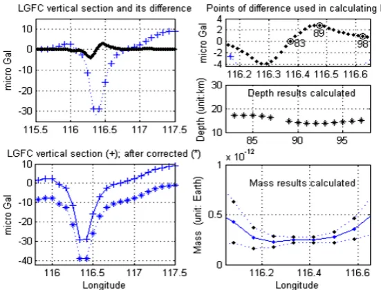
We use the LGFC (1) (1995.42-1995.67) as an example to show the detail of an H determination. Its vertical section of 5′interval at latitude 40.17˚ and the gravity change difference of 1′ interval are shown in Figure 4 top left image. The 16 points (83rd - 98th) of the time series of the latter (Figure 4 top right image) are now taking part into the calculation. The detail of part of the calculation, related to the points (86th - 91st), is presented in
Table 1. Among these 6 points, the 89th is considered as the “No.1” (distance D1) in Equation (9) whiles the other ones as the “No.2” (distance D2). Calculate one by one the ratio Kdv of the five points in considering the 89th as 100% (see the 3rd line of the table), together with their D2 (4th line), the five results of the depth H (5th line) are obtained by the equation (9). There are 16 points taken part in the calculation, but two of them, the 83rd and 88th, are used as reference points in the calculation. The derived 14 H results are now showing in Figure 4
middle right image. Their average is 15.75 ± 1.47 (km), which is the final result of the depth determination. With the location established and the depth determined, now is the time that the mass can be calculated by the observed gravity change at any point of which the distance D is known (see Equation (10)). Other points can be calculated as well (see Figure 4 lower left image). An assumed correction (−10 micro Gal) is added to the
de-rived gravity values (see Figure 4 lower left image), which is due to the incompleteness of data mentioned above. Altogether 7 of these corrected gravity change values have been used in the mass calculation; the results are shown by the solid line in Figure 4 lower right image.
Figure 4. Calculation of the depth (H) and the mass (M) in the case of LGFC(1).
Table 1. Calculating the depth (H) by the ratio Kdv.
Point No. 86 87 88 89 90 91
d/dD(△gv) (micro Gal) 2.2041 2.6179 2.8343 2.8535 2.6752 2.3403
Kdv 1.2946 1.0900 1.0067 1.0000 1.0666 1.2193
D (km) 4.42 5.84 7.26 8.68 10.40 11.52
H (km) 16.98 16.68 16.29 --- 14.84 13.96
Average of the 14 determinations (km) 15.75 ± 1.47 (km)
which is of the order of about 0.3 × 10⁻¹² (unit: Earth mass).
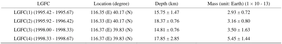
The depth and the mass derived from the other three LGFC results have also been obtained. A summary of them together is given in Table 2.
5. Discussion
In order to use gravity observations to study seismological phenomena in Beijing area, whether or not there is real detectable mass migration underground in practice is one of the important problems to be studied.
The purpose of the paper is to show evidence that there are significant LGFC in the area, and it is possible to describe the related mass migration (depth: several to 20 km; mass: of the order of 0.3 × 10⁻¹² Earth mass) by means of a point-source disturbed body. It is also possible to determine or estimate its three parameters (location, depth and mass) in using appropriate approach.
As a first step of the study, we concentrate ourselves mainly on the mass migration of which the depth is less than 20 km. In such a case, the problem can be discussed in a simplest way, considering the ground as a flat plane. Hoping that the formulae used and the results obtained will be easier to be understood and accepted by others.
In the study one understands better the importance of a gravimetric network used, especially the density of its network points. It can be seen in the contour maps (Figure 3) that the derived LGFC signal depends very much on its distance to the nearest network point. Since a LGFC signal will reduce its size to only 36% at the distance of the UDB depth H (see Figure 1),one may believe that other than the two pair LGFCs reported here, there will be quite some other ones in Beijing area that cannot be detected by the network.
higher accuracy and higher frequency. At the IAU General Assembly, Buenos Aires 1991, the Commission 19 of Rotation of the Earth made a decision of Application of Optical Astrometry Time and Latitude Programms, that optical astrometric data previously used to measure the rotation of the Earth had been shown to measure the variations in the deflection of the vertical, that the collected astrometric data contain valuable information on star positions including radio stars, and recommended that optical astrometric data continue to be collected in order to investigate the possibility of deriving long-term variations in the deflection of the vertical. In such a situation, Li et al. (2005) succeeded in observing the longitudinal component of DOV at Beijing with the accu-racy better than 0.05 seconds of arc, which can be corresponded to the variation of DOV derived from the grav-ity surveys made at the network along Beijing.
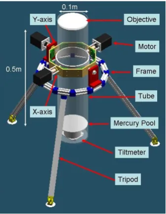
[image:7.595.86.540.331.402.2]For the optical astrometric technique, the Photographic Zenith Tube (PZT, see Figure 5) has played key role since 1900 for observations of the Earth rotation, and it also has a potential to be applied for several other ob-servations by taking advantage of automatic obob-servations with self compensation of tilt of the tube. In the pro-posed telescope ILOM (In-situ Lunar Orientation Measurement) to study lunar rotational dynamics by direct observations of the lunar rotation from the lunar surface by using a small telescope like PZT with an accuracy of 1 milli-seconds of arc in the post-SELENE mission. Another application is to obtain local gravity field on the Earth by combining deflection of the vertical measured by PZT and the position measured by GNSS (Global Navigation Satellite System). The accuracy required for this purpose is not as high as ILOM. A Bread Board Model (BBM) of the telescope for ILOM has already been developed for some experiments. See Figure 6.
Table 2. A Summary of the underground disturbed body parameters.
LGFC Location (degree) Depth (km) Mass (unit: Earth) (1 × 10 - 13)
LGFC(1) (1995.42 - 1995.67) 116.35 (E) 40.17 (N) 15.75 ± 1.47 2.93 ± 0.72
LGFC(2) (1995.92 - 1996.42) 116.33 (E) 40.17 (N) 18.37 ± 0.76 3.16 ± 0.80
LGFC(3) (1998.00 - 1998.33) 116.37 (E) 39.83 (N) 14.81 ± 0.76 3.50 ± 1.63
LGFC(4) (1998.33 - 1998.67) 116.37 (E) 39.83 (N) 17.85 ± 2.85 5.45 ± 1.44
Figure 6. Structure of BBM of the PZT (after Hanada et al.).
In the future survey at BTTZ area, both of the independent PZT and gravity methods should be used together by means of taking the advantages of them, and of validating each other. Additionally, as the relation between earthquake and the timing of a detected LGFC, it is still too early to draw any conclusion. The facts reported in the paper should be considered as some new evidence supplemented to those already reported in the past (Li et al., 2009; Li et al., 2011).
Acknowledgements
Authors thank the support of the Key Laboratory of Lunar and Deep Space, Chinese Academy of Sciences. The gravimetric data for this research is supported from BTTZ gravimetric network. A. G. Thanks to the
References
Barnes, D. F. (1966). Gravity Changes during the Alaska Earthquake. Journal of Geophysical Research, 71, 451-456. http://dx.doi.org/10.1029/JZ071i002p00451
Chen, Y., Gu, H., & Lu, Z. (1979). Variations of Gravity before and after the Haicheng Earthquake, 1975 and Tangshan Earthquake, 1976. Physics of the Earth and Planetary Interiors, 18, 330-338.
http://dx.doi.org/10.1016/0031-9201(79)90070-0
Chen, Y., Liu, K., Zheng, J., Song, S., Liu, R., Lu, H., et al. (2002). A Review of the Studies on the Relationship between Local Gravity Field Changes and Earthquakes. In S. Sun, Ed., Advances in Pure and Applied Geophysics (pp. 40-47). Me-teorology Press, Beijing.
Hanada, H., Araki, H., Tazawa, S., Tazawa, S., Tsuruta S., Noda, H., Asari, K., et al. (2012). Development of a Digital Ze-nith Telescope for Advanced Astrometry. Science China Physics, Mechanics and Astronomy, 55, 723-732.
http://dx.doi.org/10.1007/s11433-012-4673-1
Jia, M., Xing, C., & Li, H. (1998). Gravity Changes with Time in Yunnan and Beijing Observed by Absolute Gravimetry.
Bur. Grav. Int. B. Inf., 83, 50.
Jia, M., Ma, L., & Liu, S. (2006). Joint Processing and Analysis of Seismic Gravity Measurements Area around Capital of China. Acta Seismologica Sinica, 28, 408-416.
Gu, G., Kuo, J., Liu, K., Zheng, J., Lu, H., & Liu, R. (1998). Seismogenesis and Occurrence of Earthquakes as Observed by Temporally Continuous Gravity Variations in China. Chinese Science Bulletin, 43, 8-21.
http://dx.doi.org/10.1007/BF02885502
Kuo, J., & Sun, Y. (1993). Modeling Gravity Variations Caused by Dilatancies. Tectonophysics, 227, 127-143. http://dx.doi.org/10.1016/0040-1951(93)90091-W
Data in the BTTZ Region, China. Tectonophysics, 312, 267-281. http://dx.doi.org/10.1016/S0040-1951(99)00201-2 Li, H., Fu, G., Sun, S., & Xiang, A. (2000). Computation on Dynamic Gravity Changes in the Western Area of Yunnan
Province. Crust Deform Earth, 20, 60-66.
Li, H., Fu, G., & Li, Z., (2001). Plumb Line Deflection Varied with Time Obtained by Repeated Gravimetry. Acta Seis-mologica Sinica, 14, 66-71. http://dx.doi.org/10.1007/s11589-001-0162-8
Li, Z., Li, H., Li, Y. & Han, Y. (2005). Non-Tidal Variations in the Deflection of the Vertical at Beijing Observatory. J. Ge-odesy, 78, 588-593. http://dx.doi.org/10.1007/s00190-004-0421-2
Li, Z., & Li, H. (2009). Earthquake-Related Gravity Field Changes at Beijing-Tangshan Gravimetric Network. Studia Geo-phusica et Geodaetica, 53, 185-197. http://dx.doi.org/10.1007/s11200-009-0012-z
Li, Z., & Li, H. (2011). Relation between Plumb Line Variation in Tangshan Region and Underground Material Change be-fore and after Earthquakes. Acta Seismologica Sinica, 33, 817-827.
Liu, D., Li, H., & Liu, S. (1991). Processing System of Gravity Observational Data—LGADJ. In Study of Earthquake Pre-diction (Part of Crystal Deformation, Gravity) (pp. 339-350). Beijing: Press of Earthquake,(in Chinese)