Feature Selection Method for Speaker Recognition
using Neural Network
Dipen Nath
Asst. Professor, Dept. of Computer Science and IT Mangaldai College
Mangaldai, Assam, India
Sanjib Kr. Kalita, Ph.D
Asst. Professor, Dept. of Computer ScienceGauhati University Guwahti-14, Assam, India
ABSTRACT
The aim of this paper is to extract and select features from speech signal that will make it possible to have acceptable speaker recognition rate in real life. A variety of combinations among formants (F1, F2, F3), Linear Predictive Coefficients (LPC), Mel Frequency Cepstral Coefficients (MFCC) and delta- Mel Frequency Cepstral Coefficients representing features are considered and their effect in speaker recognition is observed. Two similar volume data sets with differed string (words) are considered in the present study. These two data sets are prepared taking into account two differed data sampling rates. The study reveals another interesting fact that the selection of strings in speaker enrollment process is a matter of importance for accurate result. This means that the speaker will be tested for authentication with the same string with which he was enrolled earlier during the time of his first access to the system.
General Terms
Feature Extraction and Selection, Pattern Recognition, Artificial Neural Network, Automatic Speaker Recognition
Keywords
Feature Extraction, Feed Forward Neural Network, Speaker Recognition
1.
INTRODUCTION
The uniqueness of the physiological structure of all human vocal tracts is the major factor in identifying speakers through their voice signals. Speaker recognition is the process of recognizing a person by speaker’s voice. Voice comes under the category of cognitive biometric identity for the differences in anatomical structure of the speakers. Identifying a person by means of his voice has several advantages. Remote persons can easily be authenticated using their voice signal. Based on the application, a speaker recognition system can operate in two phases, i.e. training and testing.
In the training phase, the system learns the voice characteristics of the speakers stored in the database of the system. Feature vectors that represent the voice signal of speaker are extracted and are used in the formation of reference model through the use of neural network training module. In the testing phase, same feature vectors are extractedfrom the test utterances (unknown) with the same process. Testing is the actual recognition task. The degree of their match with the reference is obtained using some matching techniques. The level of match is used to arrive at the final decision that determines whether the test utterance is acceptable or to be rejected for further processing activities.
2.
LITERATURE REVIEW
The world community of speech researchers is focusing at the automatic speech recognition (ASR) problems as a major challenge [1]. The interdisciplinary nature of speech technology constitutes another difficulty for speech research. Speech analysis and recognition tasks have been explored using different techniques and features. Some of the techniques have been listed below.
Hidden Markov Models(HMM)
Vector Quantization(VQ)
Dynamic Time Warping(DTW)
Independent Component Analysis(ICA)
Artificial Neural Network(ANN)
Fuzzy Logic in Speech Recognition
This section presents a survey about ASR using Artificial Neural Network (ANN) to provide a seminal view of how the field of ASR has evolved over the last few decades. Adjoudj Reda et. al [1] have got a speaker recognition rate up to 97% for his own data set in an attempt taking into account various data sets for MFCC and ANN architecture. Methods that are speaker dependent in nature generally involve training of a system in order to recognize individual vocabulary words that are uttered single or multiple times by a specific set of speakers [2, 3, 4]. Kshamamayee Dash et.al [3] have developed a speaker recognition system and have tested it with a speech of an unknown speaker using MFCC for feature part and feed forward ANN for classification part. The extracted features of the unknown speech are compared to the stored extracted features of each different speaker and the results they found were having efficiency 85%. They gave emphasis on collecting 100 such speech instances in future and to calculate the MFCC features for NN training to get more accurate figures for identification.
Bishnu Prasad Das et. al [5] have described a system to recognize English words corresponding to the decimal digits uttered by a set of 28 speakers. Words are classified using a combination of features based on LPC, MFCC, ZCR and STE. The recognition accuracy is shown to be 85% which is better than using features individually. The overall accuracy can be increased by combining more features of the speech samples. The filtering of the speech samples can be done through different windows like Hamming, Hanning etc.
recognition based on multilayer perceptron classifier and Euclidean distance classifier and found their recognition rates via classification as 83.38% and 96.18% respectively. Lajish V. L et.al [6] had modelled the speaker identity based on the non-linearity principles of speech, which are normally not considered in conventional feature extraction methodologies. The speaker identification experiments are conducted based on Phase Space Point Distribution (PSPD) firstly. The PSPD features obtained from five vowels are used for speaker identification purpose using the feed forward multi layer perceptron. The experiment is repeated by taking different combinations of features like PSPD, MFCC, pitch and first formant frequency. Experiments indicate that the firstly proposed approach by itself is still below (31.60%) than that of MFCC features (46.21%). The combined approach in which the PSPD features are used with MFCC, pitch and first formant frequency offers sufficient improvement in speaker identification (on an average of 83.40%) accuracy.
3.
THEORETICAL BACKGROUND
3.1
Formant and LPC
LPC analyses speech signal through formant estimations by removing their effects from the speech signal, and it estimates the intensity and frequency of the remaining low sounds [7, 8, 9, 10]. This process of removing formants is called inverse filtering, and the remaining signal is called the residue. Each sample of a signal is expressed as a linear combination of the previous samples in LPC. This equation is termed as linear predictor and hence called as linear predictive coding. The coefficients of the difference equation characterize the formants.
A predictor polynomial, which is generally defined as the Fourier transform of the corresponding second order predictor is given by [8, 9, 10]
w j k jw k jw
k e e e
A 2
1 )
(
(1)
where,
k
and k
are the real valued prediction coefficients. From equation (1), we get
) 2 cos( 2 cos ) 1 ( 2 1 | ) (
| 2 2 2
k k k k k jw k e
A
2 2 2 2 2 2 2 4 ) 1 ( cos 4 4 ) 1 ( ) 1 ( k k k k k k k k k (2) The parameter
k
determines the bandwidth of the resonator and defined as negative logarithm of
. )] ( ).[
( jw 2
k k A e
The formant frequency is given by
k k k
F
4 ) 1 ( arccos 1
(3)
Using equation (1), the corresponding predictor error can be written as
) 2 ( 2 ) 1 ( ) 1 ( 2 ) 0 ( ) 1 ( ) , | , ( 2 2 1 k k k k k k k k k k k k r r r E (4)
where, ()
k
r are the autocorrelation coefficients where =0, 1, 2. Also
|
cos
|
1
,
and thus the values of
k and k are taken as- 4 1 2 2 k k k
(5)
3.2
MFCC
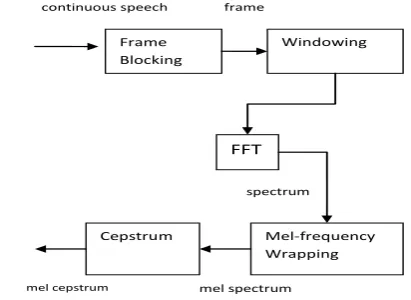
The earlier methods of feature extraction preferably used the LPC and Formant frequency estimations [8, 11, 12]. But these days Mel Frequency Cepstral Coefficient (MFCC) is found to be widely used in signal and speech processing. These coefficients have an immense success in speech processing application. MFCCs are parametric representations (at considerably lower information rate) extracted from speech waveform. A flowchart depicting the steps in MFCC processing [8, 13, 14] is mentioned below in Figure-1.
Frame Blocking
The speech signal is divided into blocks of N samples and the adjacent blocks are separated by M (where M < N). The first block consists of first N samples and the second frame begins M samples after the first block. Thus the overlapping value is N-M. This process continues until the entire speech signal comes to an end. Typical value of N=256 (which is equivalent to ~ 30 millisecond windowing) and M=100 [12].
Windowing
Each individual block is then windowed so that the signal discontinuities can be minimized at the beginning and end of each block. The intention behind doing this is to minimize the spectral distortion and to narrowthe signal to zero at the beginning and end of each frame. The window is defined as
w
(
n
),
0
n
N
1
, where N is the number of samples in each block. The output of the windowing process can be defined as [4, 5]1
0
),
(
)
(
)
(
n
x
n
w
n
n
N
y
l l (6)Fast Fourier Transform (FFT)
FFT is a process of converting each block or frame of N samples from the time domain into frequency domain. This algorithm implements the Discrete Fourier Transform (DFT), which is defined on the set of N samples {xn} as
Frame Blocking Windowing FFT Mel-frequency Wrapping Cepstrum mel spectrum mel cepstrum spectrum
[image:2.595.327.533.294.444.2]continuous speech frame
1
0
/
2 , 0,1,2,..., 1
N
n
N kn j n
k x e k N
X (7)
The output of this step is referred to as spectrum or periodogram.
Mel-frequency wrapping
It is observed in the psychophysical studies that human perception of the frequency contents of sound for speech signal follows a nonlinear scale. That is why, for each tone with an actual frequency, say f Hz, a subjective pitch is measured in Mel scale. The Mel frequency scale is linear frequency spacing below 1000 Hz and a logarithmic spacing above 1000 Hz [4, 5]. Subjective spectrums can be simulated by using a filter bank that are spaced uniformly on the Mel scale.
Cepstrum calculation
Cepstrum is derived from the Fourier Transform of the recorded speech signal. Due to logarithmic positioning of the frequency bands in MFCC, it approximates the human auditory system more closely than any other system. These coefficients allow better processing of data, where the calculation of Mel cepstrum is same as the real cepstrum, except the Mel cepstrum frequency scale is wrapped to keep up a correspondence to the Mel scale.
3.3 Feed Forward ANN
Feed forward artificial neural network (FFANN) [1, 12, 14, 15, 16] is a widely used classification technique, whereas non- linear methods of discrimination developed in the statistical field are much less widely known. Neural networks emerge as a flexible non parametric classification method, which is used frequently to classify via regression or even mean square error. Feed forward neural networks provide a flexible way to generalize regression. In our study, we have implemented the simplest and the most common form with one hidden layer.
3.4
Levenberg-Marquardt Algorithm
The Levenberg-Marquardt Algorithm (LMA) is an algorithm to solve generic curve-fitting problems. Nonlinear least squares problems arise for non linearity in the parameters. It improves the parameter values iteratively to reduce the sum of the squares of the errors between the function and the measured data points. A combination of two methods, namely, the Gradient Descent method and the Gauss-Newton method is used in the Levenberg-Marquardt curve fitting method. In the gradient descent method, the sum of the squared errors is reduced by updating the parameters in the direction of the greatest reduction of the least squares objective. But in Gauss-Newton method, the sum of the squared errors is reduced by assuming the least squares function to be locally quadratic, and finding the minimum of the quadratic [2].
The Levenberg-Marquardt method acts like a gradient-descent method, when the parameters are far from their optimal value and when the parameters are close to their optimal value, it acts like Gauss-Newton method. MATLAB is used to train the proposed network by implementing LMA as back propagation algorithm. LMA is a popular supervised category algorithm [2, 17, 18], although it requires more memory than other such algorithms.
Validation vectors are used to stop training early if the network fails to improve or remains the same, whereas test vectors are used for checking whether the network is generalizing well or not, but it does not have any effect on training.
3.5
Speaker Recognition
Speaker recognition basically focuses on identification task [19, 20]. Speaker identification (SI) deals in identifying the unknown speaker from a set of known speakers (closed set SI). A speaker recognition system uses the following modules.
Pre-processing
Sampled signal is converted into a set of features characterizing the properties of the speaker, which is repeated both in training and testing phases.Speaker modeling
This part performs a sort of reduction in features by modeling the distribution of the feature vectors.
Speaker database
Speaker models are stored here for confidence measure.
Decision logic
F
inally identifies the new comer by comparing it with all stored models in the database and selects the best match.4.
EXPERIMENTAL SETUP
4.1
Speech Database
The first data set is recorded in 16KHz sampling frequency whereas the second data set is recorded with a sampling frequency of 44.1KHz. Words considered for the first set are ‘Green’, ‘Indigo’ and ‘Red’ whereas words taken for the second data set are ‘Logoff’, ‘Restart’ and ‘Shutdown’. A total of six speakers are involved in preparation of both the data sets. Male-age-34, male-age-15 & female-age-14 and Male-age-34, male-age-24 & female-age-28 are the corresponding contributors for the Data Set-1 and Data Set-2 respectively.
One single data set is composed of two males and one female with three different words. That means six males and two females have contributed to prepare the whole dataset containing six words. So we have [(50x3) x3]=450 utterances in each data set. The experiment has been carried out with Intel (R) core (TM) i-5 2430M CPU @2.40 GHz 2.40 GHz processor and 3.00 GB RAM. Windows 7 Ultimate (32-bit o/s) and MATLAB version 7.11.0 (R2010b) is used for the experiment part and Goldwave Version 5.58 is used for recording of the sound samples.
4.2
Network Architecture
dataset-1(450 utterances) are used for the network training, validation and testing procedures respectively. Same is the case for dataset-2 for another 450 utterances. Finally after getting satisfactory regression results, we select that network for future recognition task. A total of 90 utterances (30 utterances against each word) are considered for recognition process for each data set in order to calculate the final recognition rates considering 0.8 as the threshold value. The experiment was repeated for several times to fix the threshold value. The performance of the recognizer has been depicted in Table-1 and Table-2 in terms of the accuracy in recognition.
5.
RESULT AND DISCUSSION
The features Formants (F1,F2,F3), LPC, MFCC, ΔMFCC, Formant + LPC, Formant + LPC + MFCC, Formant + LPC + MFCC + ΔMFCC and LPC + MFCC + ΔMFCC are studied here. Data Set-1 is prepared taking into account the words ‘Red’, ‘In-di-go’, ‘Green’ spoken by 3 speakers
[image:4.595.196.423.314.770.2]and Data Set-2 is prepared taking into account the words ‘Log-off’, ‘Re-start’ and ‘Shut-down’ spoken by another 3 speakers. But if we study Table-1 and Table-2, we come into one conclusion that the word ‘indigo’ is giving higher performance in terms of speaker recognition for Data Set-1 and the words ‘Re-start’ and ‘Shut -down’ are giving higher performances in terms of speaker recognition for Data Set-2. It is focusing on a factual idea that strings (words) containing more phonemic contents perform well while comparing with short length and less phonemic strings in terms of recognition. The features that are found to be invariant in both the experiments with different data sets and different speakers are MFCC, Formant + LPC, Formant + LPC + MFCC + ΔMFCC and LPC+MFCC+ ΔMFCC. But amongst them the ’Formant + LPC’ combination is found to be close to 100% recognition as compared to other three selections. So this feature is supposed to be a better choice in speaker recognition. Table-3, Table-4, Figure-2 and Figure-3 are the evidences in favour of the above inferences.
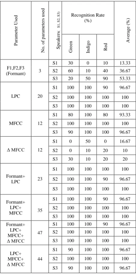
Table 1: Comparison among speakers w.r.t. various feature set for Data Set-1
P
ar
ame
te
r
U
se
d
N
o
.
o
f
p
ar
am
et
er
s
u
se
d
S
p
ea
k
er
s
(
S
1
,
S
2,
S
3) Recognition Rate
(%)
A
v
er
ag
e
(%)
G
re
en
In
d
ig
o
R
ed
F1,F2,F3 (Formant) 3
S1 30 0 10 13.33
S2 60 10 40 36.67
S3 20 50 90 53.33
LPC 20
S1 100 100 90 96.67
S2 100 100 100 100
S3 100 100 100 100
MFCC 12
S1 80 100 80 93.33
S2 100 100 100 100
S3 90 100 100 96.67
Δ MFCC 12
S1 0 50 0 16.67
S2 0 10 20 10
S3 30 10 20 20
Formant+
LPC 23
S1 100 100 100 100
S2 100 100 90 96.67
S3 100 100 100 100
Formant+ LPC+
MFCC 35
S1 100 100 90 96.67
S2 100 100 100 100
S3 100 100 100 100
Formant+ LPC+ MFCC+ Δ MFCC
47
S1 100 100 90 96.67
S2 100 100 100 100
S3 100 100 100 100
LPC+ MFCC+ Δ MFCC 44
S1 90 100 100 96.67
S2 100 100 100 100
Table 2: Comparison among speakers w.r.t. various feature set for Data Set-2
P
ara
m
eter Use
d
No
.
o
f
p
ara
m
eters
u
se
d
S
p
ea
k
ers
(
S
1
,
S
2
,
S
3
)
Recognition Rate (%)
Av
era
g
e
(%
)
Lo
g
o
ff
Re
sta
rt
S
h
u
td
o
w
n
F1,F2,F3 (Formant) 3
S1 30 60 50 46.67
S2 80 70 10 53.33
S3 90 100 100 96.67
LPC 50
S1 50 0 30 26.67
S2 100 100 80 93.33
S3 90 100 90 93.33
MFCC 12
S1 60 100 100 86.67
S2 100 100 100 100
S3 100 100 100 100
Δ MFCC 12
S1 0 0 0 0
S2 70 70 90 76.67
S3 10 20 20 16.67
Formant+
LPC 53
S1 100 100 100 100
S2 100 100 100 100
S3 100 100 100 100
Formant+ LPC+
MFCC 65
S1 80 40 100 73.33
S2 90 80 80 83.33
S3 100 100 100 100
Formant+ LPC+ MFCC+ Δ MFCC
77
S1 100 100 100 100
S2 90 100 100 96.67
S3 100 90 100 96.67
LPC+ MFCC+ Δ MFCC
74
S1 100 100 100 100
S2 90 100 100 96.67
S3 100 100 100 100
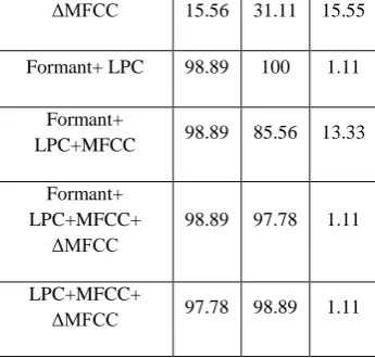
Table 3- Performance Comparison among both Data Sets
Features Used
Da
ta S
et
-1
Re
co
g
n
it
io
n
(%
)
Da
ta
S
et
-2
Re
co
g
n
it
io
n
(%
)
Ga
p
(%
)
Formant 34.44 65.56 31.12
LPC 98.89 71.11 27.78
MFCC 96.67 95.56 1.11
ΔMFCC 15.56 31.11 15.55
Formant+ LPC 98.89 100 1.11
Formant+
LPC+MFCC 98.89 85.56 13.33
Formant+ LPC+MFCC+
ΔMFCC
98.89 97.78 1.11
LPC+MFCC+
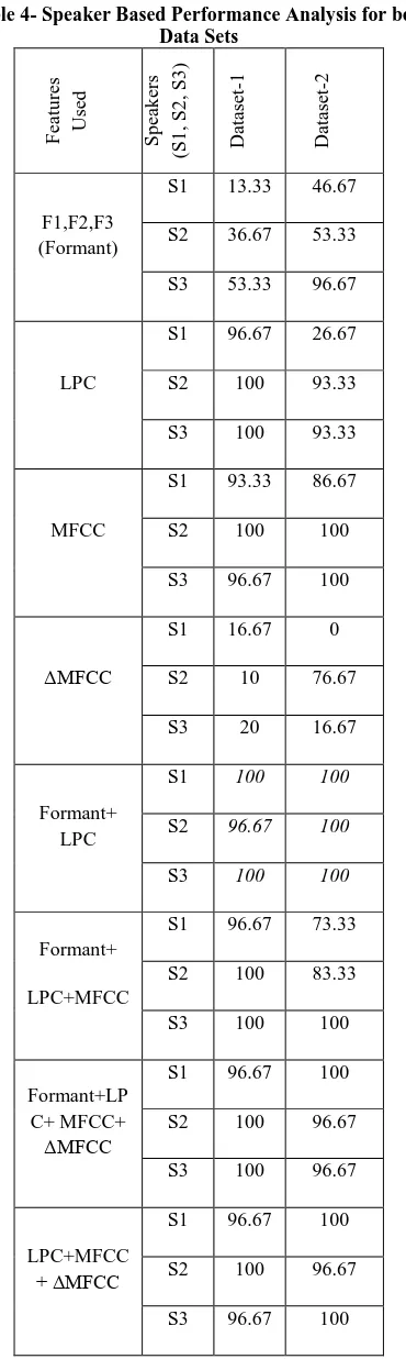
[image:5.595.348.521.591.756.2]Table 4- Speaker Based Performance Analysis for both Data Sets
F
ea
tu
re
s
Us
ed
S
p
ea
k
ers
(S
1
,
S
2
,
S
3
)
Da
tas
et
-1
Da
tas
et
-2
F1,F2,F3 (Formant)
S1 13.33 46.67
S2 36.67 53.33
S3 53.33 96.67
LPC
S1 96.67 26.67
S2 100 93.33
S3 100 93.33
MFCC
S1 93.33 86.67
S2 100 100
S3 96.67 100
ΔMFCC
S1 16.67 0
S2 10 76.67
S3 20 16.67
Formant+ LPC
S1 100 100
S2 96.67 100
S3 100 100
Formant+
LPC+MFCC
S1 96.67 73.33
S2 100 83.33
S3 100 100
Formant+LP C+ MFCC+ ΔMFCC
S1 96.67 100
S2 100 96.67
S3 100 96.67
LPC+MFCC + ΔMFCC
S1 96.67 100
S2 100 96.67
S3 96.67 100
6.
CONCLUSION & FUTURE WORK
The efficiency of the recognizer has been examined with different combination of features. The feature Formant+LPC is found to be the optimal combination feature set amongst the other three high accuracy feature sets (i.e. MFCC, Formant+LPC+MFCC+ΔMFCC and
LPC+MFCC+ΔMFCC) for higher speaker recognition rate that reaches to a maximum of 100% speaker recognition with a very closer gap in recognition performance between the two datasets (i.e. Dataset-1 and Dataset-2). Two different experiments with different data sets with different sampling rates give us strong evidences for concluding the study to support Formant+LPC feature for a very higher speaker recognition rate. Also the strings with more phonemic contents are found to be a better choice for higher speaker recognition rate.
[image:6.595.327.565.236.409.2]This work can be extended to distinguish among male and female speakers and the entire study can again be done using some standard data sets and compare the end results, which will help formulating few new results.
[image:6.595.327.563.455.647.2]Figure 2- Performance Comparison among both Data Sets
Figure 3- Speaker Based Performance Analysis for both Data Sets
7.
ACKNOWLEDGMENT
8.
REFERRENCES
[1] Adjoudj Reda, Boukelif Aoued, “Artificial Neural Network & Mel-Frequency Cepstrum Coefficients-Based Speaker Recognition”, 3rd International Conference: Sciences of Electronic, Technologies of Information and Telecommunications--TUNISIA, March 27-31, 2005
[2] Mark K. Transtrum and James P. Sethna “Improvements to the Levenberg-Marquardt algorithm for nonlinear least-squares minimization,” Preprint submitted to Journal of Computational Physics, January 30, 2012.
[3] Kshamamayee Dash, Debananda Padhi, Bhoomika Panda, Prof. Sanghamitra Mohanty, “Speaker Identification using Mel Frequency Cepstral Coefficient and BPNN”, International Journal of Advanced Research in Computer Science and Software Engineering, Volume 2, Issue 4, ISSN: 2277 128X, April 2012
[4] Praveen N, Tessamma Thomas, “Text dependent speaker recognition using MFCC features and BPANN”, International Journal of Computer Applications (0975 – 8887), Volume 74– No.5, July 2013
[5] Bishnu Prasad Das, Ranjan Parekh, “Recognition of Isolated Words using Features based on LPC, MFCC, ZCR and STE with Neural Network Classifiers”, International Journal of Modern Engineering Research (IJMER) ,Vol.2, Issue.3, pp-854-858 [ISSN: 2249-6645], May-June 2012
[6] Lajish V.L , Sunil Kumar R.K and Vivek P, “Speaker identification using a nonlinear speech model and ANN”, International Journal of Advanced Information Technology (IJAIT) Vol. 2, No.5, October 2012
[7] Thiang, Suryo Wijoyo. “Speech Recognition Using Linear Predictive Coding and Artificial Neural Network for Controlling Movement of Mobile Robot”. 2011 International Conference on Information and Electronics Engineering IPCSIT vol.6 © (2011) IACSIT Press, Singapore, 2011 [8] Talukdar, P. H., Bhattacharjee, U., Goswami, C. K. ,
Barman, J., “Cepstral Measure of Boro Vowels through LPC-Analysis”, Journal of the CSI, Vol. 34 No 1, Jan – Mar, 2004
[9] Kalita S.K., Dutta R., and Talukdar P. H., “A spectral analysis of Bodo and Assamese vowels”, Abstracts
3rd International Conference on “Computers and Devices for Communication”. CODEC – 06, Kolkata, India, pp. 41, 2006
[10]Braman, J., Kalita, S., Talukdar, P. H., “Features extraction of bodo vowels through lpc-analysis”, Proceedings of Frontiers of Research on Speech and Music (FRMS-2004), 2004
[11]Hasan Rashidul, Jamil Mustafa, Rabbani Golam, Rahman Saifur, “Speaker identification using mel frequency cepstral coefficients”, 3rd International Conference on Electrical & Computer Engineering, Dhaka, Bangladesh, ICECE 2004, 28-30 December 2004
[12]Rabiner L., Juang B. H. and Yegnanarayana B. – “Fundamentals of Speech Processing”, Pearson Education, ISBN 978-81-775-8560-5, 2011
[13]D.Ripley, “Neural Networks and Related Methods for Classification”, Journal of the Royal Statistical Society. Series B (Methodological), Vol. 56, No. 3(1994), pp. 409-456, 1994
[14]Rabiner L. and Juang B. H. – “Fundamental of Speech Processing”, Prentice-Hall, 1993
[15]Bishop, C., “Neural Networks for Pattern Recognition”, Oxford University Press, Oxford, 1995 [16]Haykin, S., “Neural Networks - A Comprehensive
Foundation”, 2nd
ed. Prentice-Hall, Englewood Cliffs, 1998
[17]K. Levenberg. “A Method for the Solution of Certain Non-Linear Problems in Least Squares”. The Quarterly of Applied Mathematics, 2: 164-168, 1994 [18]M.I.A. Lourakis., “A brief description of the
Levenberg-Marquardt algorithm” implemented by levmar, Technical Report, Institute of Computer Science, Foundation for Research and Technology, - Hellas, 2005
[19]Vibha Tiwari, “MFCC and its applications in speaker recognition”, International Journal on Emerging Technologies 1(1): 19-22(2010) ISSN: 0975-8364, 2010