An Efficient Hybrid Image Coding Scheme Combining Wavelets, Neural Networks and Differential Pulse Code Modulation for Effectual Image Compression

41

An Efficient Hybrid Image Coding Scheme Combining

Wavelets, Neural Networks and Differential Pulse Code

Modulation for Effectual Image Compression

Sridhar Siripurapu

Faculty, ECE

Lendi Institute of Engg&Techn Vizianagaram

Rajesh Kumar P

Associate Professor, ECE AU College of Engg

Visakhapatnam

Ramanaiah K V

Associate Professor, ECE YSR Engineering College of

YOGI VEMANA University

ABSTRACT

Large images consume more storage space needing high data rates for transmission demanding the innovation of efficient image compression systems. Owing to the massive parallel architecture and generalization ability of neural networks to memorize inputs even on untrained data, the computational simplicity of wavelets, ability of Differential Pulse Code Modulation (DPCM) to reduce the unused or redundant bits in the information, in this paper an hybrid image compression system combining the advantages of wavelets and neural networks is implemented along with Differential Pulse Code Modulation based on the predicted sample values. Scalar quantization and Huffman encoding schemes are used as well for compressing different sub bands i.e the low frequency band coefficients are compressed by the DPCM while the high frequency band coefficients are compressed using neural networks. Satisfactory reconstructed images with increased bit rates and large Peak Signal to Noise Ratio (PSNR) can be achieved with this scheme. Wavelet transform eliminates the blocking artefacts’ associated with cosine transform and neural networks minimize the Mean Square Error (MSE).Empirical analysis and metrics calculation is performed for the sake of relative analysis.

General Terms

Artificial Neural Networks, Fidelity, Mean Square Error, Peak Signal to Noise Ratio, Quantization and Huffman encoding.

Keywords

Differential Pulse Code Modulation, Error Backpropagation, Haar Wavelet, Image Compression.

1.

INTRODUCTION

The development of high performance computing and communication opened up tremendous opportunities in different telecommunication applications and multi-media computer services like videoconferencing, interactive education etc. Image compression is a context where images of different types and different sizes are compressed using different methodologies while data compression is the only solution to meet large storage space requirements and ever growing bandwidth requirements [1].

Since images can be regarded as two dimensional signals, many digital Image compression techniques for one dimensional signals can be extended to images with relative ease to exploit the correlations between the neighboring pixels because a still image contains large amount of spatial

redundancy in plain areas where adjacent pixels or elements have almost the same values. Additionally [5] any still image contains subjective redundancy i.e. determined by properties of human visual system by presenting a level of tolerance to the distortion based on the image content, Consequently pixels must not always be reproduced exactly that the human visual system may at all times fail to detect the difference between original image and reproduced image. Existing traditional techniques reduces the Coding Redundancy, Interpixel Redundancy and Psycho visual Redundancy, [2] additionally new soft computing technologies like Neural Networks are developed for image compression. Parallelism, Learning capabilities, Noise Suppression, Transform extraction and Optimized Approximations are few valid reasons encouraging researchers to use artificial neural networks in combination with wavelets for image compression approach. The proposed hybrid compression methodology eliminates all forms of redundancies in the images by combining both the lossy and lossless compression techniques.

This paper is organized as follows. Section 2 details various image compression methodologies employed for the proposed architecture- the Haar wavelet transform, DPCM, Neural networks etc. Section 3, discusses the backpropagation algorithm for training neural networks. Section 4 explains the proposed hybrid architecture of image encoding and decoding system. Sections 5and 6, elaborates the Experimental analysis and results of implementation. Conclusions are drawn in Section 7 and summarized.

2.

IMAGE COMPRESSION MODELS

42 gradual spatial variation of brightness from regions with faster

variations in brightness at edges of the image [4]. Few other lossy compression techniques are Vector quantization, Fractal coding, Block Truncation coding and Sub band coding etc.

2.1

Wavelet Transforms

Often [16][23] signal processing in time domain require information like frequency, Mathematical transforms translate the signal information into different representations i.e the Fourier transform converts signal between the time and frequency domains, but Fourier transform failed to provide frequency information at particular times. This problem is solved by the window based Short Term Fourier Transform (STFT) technique in which different parts of a signal are viewed. For a given window in time the frequencies can be viewed. As the signal resolution is improved in time domain its frequency resolution gets worse. Hence a method of multiresolution is needed allowing certain parts of the signal to be resolved well in time and other parts to be resolved well in frequency, rather than examining entire signals through the same window. [17] [21]Different parts of the wave are viewed through different size windows where high frequency parts of the signal use a small window to give good time resolution while the low frequency parts use a big window to get good frequency information. Wavelet transform has high décorrelation and energy compaction properties. Blocking artifacts and mosquito noise are also absent in wavelet based coder, distortion due to aliasing can be eliminated by designing proper filters. Wavelet transform is also better suited to human visual system since its basis functions are localized in frequency and space. These properties made wavelets suitable for image compression.

Wavelet transform analysis [24] represents an image as a sum of wavelet functions with different locations and scales. Wavelet decomposition of an image involves a pair of waveforms to represent, the high frequencies Correspond to the detailed parts of an image (wavelet Function) showing the Vertical, Horizontal and Diagonal details in the image and the low frequencies or Smooth parts of an image (scaling function) correspond to the approximation coefficients. [16] If the high frequency coefficients are small in number they can be set to zero without significantly changing the image, the value below which these details can be considered small enough to be set to zero is known as Threshold. If the numbers of zeros are greater then greater compression can be achieved. [25] The amount of information retained by an image after compression and decompression is known as energy retained which is proportional to the sum of the squares of the pixel values. If the energy retained is 100% then the compression is lossless and the image can be reconstructed exactly. This occurs when the threshold value is set to zero, meaning that the detail has not been changed. If any values are changed then energy will be lost leading to a lossy compression. Ideally, during compression the number of zeros and the energy retention will be as high as possible. Wavelet transforms are broadly classified as Continuous and discrete wavelet transforms. For long signals continuous wavelet transforms are time consuming, to overcome this complexity, discrete wavelet transforms are introduced. Discrete wavelet transforms (DWT) can be implemented through sub band coding. DWT is useful because it can localize signals in time and scale, whereas the DFT or DCT can localize signals in the frequency domain. The DWT is obtained by filtering the signal through a series of digital

filters at different scales. The scaling is done by means of sampling by changing the signal resolution [13].

2.1.1

HAAR Wavelet

Alfred Haar proposed Haar matrix –a simplest possible wavelet and a fast transform [15-16] in the year 1909.In mathematics, Haar wavelet is a sequence of rescaled “square-shaped” functions which together form a wavelet family or basis. The technical disadvantage of Haar wavelet is that it is not continuous and therefore not differentiable and resembles a step function. This property can, however, be an advantage for the analysis of signals with sudden transitions, such as monitoring of tool failure in machines. It represents same wavelet as Daubechies 1[13]

Figure 1. Scaling and Wavelet functions of HAAR

The properties of HAAR Transform are enumerated as under:

a) Haar Transform is real and orthogonal Hr=Hr*

b) The basis vectors of Haar matrix are sequence Ordered.

c) Haar transform has poor energy Compaction for Images.

d) Original signal is Split into a low and a high Frequency part and Enabling filters without Duplicating information.

e) Symmetric filters used for obtaining linear phase.

2.2

Differential Pulse Code Modulation

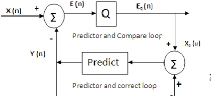
43

Figure 2. DPCM Encoder

The difference of the original image data, x (n), and prediction image data, y(n) is called estimation residual, e(n). So

e (n) = x (n) – y (n) (1)

Is quantized to yield

e Q (n) = x (n) + q (n) (2)

Where q (n) is the quantization error and eq (n) is quantized

signal and

q (n) = eq (n) – e (n) (3)

(4)

Here b is number of bits. Imax (Simg ) max is maximum value of an image signal. The prediction output y (n) is fed back to its input so that the predictor input xs (n) is

xs (n) = y (n) + eq (n) (5) =x (n) – e (n) + eq (n)

= x (n) + q (n)

This shows xs (n) is quantized version of x (n). The prediction

input is indeed xs (n), as assumed.

2.3

Neural Networks

[1] The motivation for the development of neural networks arises from a desire to develop an artificial system to perform “intelligent” tasks similar to the ones performed by human brain. A neural network is a nonlinear system and a powerful data modeling computing tool for solving optimization problems. Owing to the parallel mechanism approach, neural network can solve large scale problems efficiently to obtain an optimal solution

[6] [8] The advantage of neural networks lies in the following theoretical aspects. First, neural networks are data driven self adaptive i.e they adjust themselves to data without any explicit specification of the functional or distributional form of the underlying model. Second, neural networks are universal function approximators and can approximate any function with arbitrary accuracy. Third neural networks can estimate the probabilities to perform statistical analysis. Fourth, neural networks are fault tolerant via redundant information coding. Fifth, capabilities of neural networks can be retained despite major network damage with corresponding degradation of performance. Finally, neural networks are flexible to model the real world complex relationships.

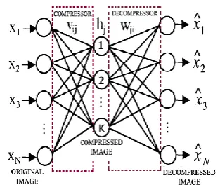
Feed forward neural network is the simplest ANN architecture in terms of the direction of information flow, many neural network architectures are variations of the feed forward neural networks consisting of a number of layers. Each layer in turn contains a number of synapses. Traditionally, the first layer is considered input layer, the last one the output layer and the one in between is regarded the hidden layer.

Figure 3. Basic Image Compression using ANN

[9] In this type of architecture input from large number of neurons is fed to a less number of hidden layer neurons, which is further fed to large number neurons in the output layer of the network. The number of connections between any two layers in the NN can be calculated by multiplying the total number of neurons of the two layers, then adding the number of bias neurons connections of the second layer (bias connections of a layer is equal to the number of layer neurons) .If there are Ni neurons in the input layer, Nh neurons in the hidden layer and No neurons in the output layer, the total number of connections is given by the equation:

Network Size :(Nw)= [( Ni*Nh )+Nh ]+[( Nh*No )+No ]

[4] Multi layered feed forward neural networks normally provide high compression ratio by exploiting correlation between pixels within a pixel patch and correlation between the pixel patches themselves thereby allowing simultaneous processing of large amounts of data to reduce the training and operation time i.e. compression-decompression time. Backpropagation (BP) is one broadly used learning method for multi-layered feed forward hierarchal neural network [2].There are two practical approaches for implementing the Backpropagation algorithm: Batch training approach and Concurrent (online updating) approach. Corresponding to the standard gradient method, batch updating method accumulates the weight corrections over all the training samples before actually performing the update while the concurrent approach updates the networks weights immediately after each training sample is fed[3,6].

3.

LEVENBERG MARQUARDT

ALGORITHM

Artificial neural networks are well suited for image compression, as they pre-process input patterns to produce compressed patterns providing sufficient compression rates while preserving the information security as well from the external environment. There are different algorithms [4] for training the neural networks, like Scaled conjugate gradient, Levenberg-Marquardt (Backpropagation), Bayesian

regulation, Resilient Backpropagation etc. In the proposed architecture of image compression system neural networks trained with LM algorithm are used for image compression, in addition discrete wavelet transform, DPCM, Quantization, and Huffman coding etc are few other compression techniques employed for eliminating the redundancies.

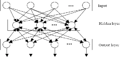
[4] [8][9] Levenberg-Marquardt (Backpropagation) algorithm is the most widely used neural network algorithms applicable to the problems of data compression. It is one of the common supervised training methods based on error-correction learning rule. Error is propagated in the forward and backward direction through the layers of the network, In the forward pass the input vectors are applied to the nodes of the network and the effect propagates through the network layer by layer producing an output response, in the forward direction the weights of the network remain fixed, while in the backward direction the layer weights are adjusted in proportion to error correction rule. Training involves iterative updating of weights to minimize the mean square error (which is the difference between the actual network responses and desired. The error signal is propagated in the reverse direction for updating the weights in a direction to minimize the error and reduce the distance between the actual response and desired response of the network, learning rate and momentum factor are the two parameters that can be varied for adjusting the weights to minimize the error and dampen the oscillations.

Figure 4. Architecture of Backpropagation network

For networks having more than one hidden layer Backpropagation algorithm converges slowly due to the saturating nature of the activation functions used for both hidden and output layers, because the descent gradient takes a very small value, though the output error is large, leading to a minute progress in the weights adjustment.

4.

PROPOSED IMAGE ENCODING /

DECODING METHODOLOGY

The proposed hybrid image encoding and decoding scheme combines Discrete Wavelet Transform, Neural Networks, Differential Pulse Code Modulation, Quantization and Huffman encoding techniques [10], The compression process is initiated considering a series of standard de-facto images. Performing a two level HAAR wavelet decomposition, the low frequency band coefficients are then compressed in the DPCM encoder while the high frequency band coefficients are compressed in a parallel arrangement of neural networks five in number. Subsequent stages involves quantization of the compressed neural networks outputs and combining the same with DPCM encoded data followed by Huffman encoding the combined coefficients of DPCM and quantized neural network outputs there by generating the compressed output. Decompression involves the reverse operations of Huffman

decoding, inverse quantization, IDPCM, Neural networks and IDWT. The approach adopted in this work differs from other schemes by taking into consideration different families of wavelets in the initial stages of compression; even the detailed coefficients of first level decomposition are used for encoding for ensuring good quality reconstructed image with better metrics. Balanced neural networks are used for compressing low frequency coefficients; also band1 approximation coefficients are eliminated from scalar quantization for the second time after being quantized initially in DPCM encoding there by reducing information loss, as quantization is a lossy and irreversible operation. Several bench mark images are considered for experimentation but a few like Cameraman, Peppers, Person, Office, Horse etc of size 256 x 256 are discussed in this work (for lack of space) as the methodology remains same for all the images generating different metrics values based on the content or relevancy of information present in the images .

4.1

Image Compression Scheme

An image of size 256 x 256 is decomposed into seven frequency bands a2, h2, v2, d2, h1, v1 and d1 with different resolutions after performing the two level wavelet decomposition using HAAR wavelet. The first level of decomposition produces approximation coefficients a1 and three detail coefficients namely h1, v1, d1 with resolutions of 128 X 128. The first level approximation coefficients are now decomposed in the second level generating a2, h2, v2, d2 coefficients of resolutions 64 x 64 totalling to a number of seven bands of coefficients. The first band in the second level decomposition contains the Approximation coefficients a2, these are the high-scale low frequency components of the signal containing significant information similarly the second, third and fourth bands represent the detail coefficients that are low-scale, high frequency components of the signal.

45 The band1 low frequency approximation coefficients a2 after

second level of decomposition are compressed using DPCM to reduce the inter pixel redundancy. In DPCM, Depending upon previous pixel information we can predict the next pixel, the difference between current pixel and predicted pixel is given to optimal quantizer which reduces the granular noise and slope over load noise. Finally we get the error output from DPCM the error images corresponding to various benchmark input images used for testing are shown in the results section. The detailed coefficients h2, v2, d2, h1, v1 after second level

of decomposition are encoded using five different neural networks of different neurons in each of the layers. However each neural network is trained with the LM algorithm. The compressed coefficients of the hidden layer output layers are then scalar quantized to eliminate the psycho visual redundancy, quantized bits along with DPCM encoded data are combined and Huffman encoded for eliminating the coding redundancy

The first level diagonal coefficients d1 obtained after the initial wavelet decomposition are discarded in the present work as they contain no useful data.

Figure 5. Proposed Image Compression Architecture

4.2

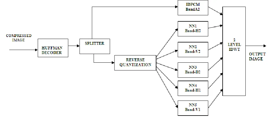
Image Decompression Scheme

Decompression process as shown in Fig. 6, involves giving Huffman encoded compressed image to the Huffman decoder, where the reconstructed bit streams are reverse quantized after splitting the values of band-1 and remaining 5 bands (band 2 to band 6). Here band-1 is the compressed low frequency band while bands 2 to 6 are compressed high frequency bands. The compressed low frequency band-1 coefficients are given to inverse DPCM and the compressed high frequency bands coefficients are given to the output layers of the respective neural networks. The reconstructed sub bands are joined for reconstruction by performing Inverse Discrete Wavelet Transform (IDWT), whose output is the desired reconstructed image.

5.

EXPERIMENTAL ANALYSIS

Experiments are conducted on several bench mark images, for every image, the coefficients of band-1 are encoded with

DPCM, coefficients of band2, and band3 and band 4 are encoded with neural networks of 16-14-16 dimensions having 16 input neurons 16 output neurons and 14 hidden neurons. While neural networks of dimensions 16-8-16 are used for coefficients of band5 and band6 ensuring more amount of compression ratio since band5 and band6 represent horizontal and vertical coefficients with less amount of significant details. The compressed hidden layer outputs of neural networks are scalar quantized and combined with DPCM encoded data which is further Huffman encoded.

6.

RESULTS

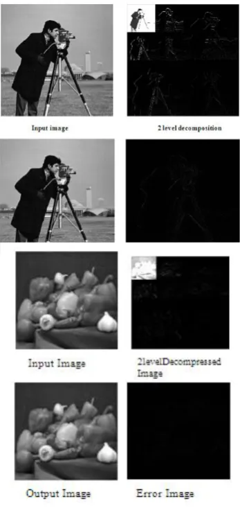
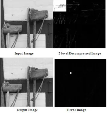
Images corresponding to the input data, 2-level DWT compressed data, system output data and error data are shown in this section. Metrics obtained like PSNR and MSE are tabulated for relative analysis.

Table 2. Results of Peppers Image Figure 7. Cameraman image

Table 1. Results of Cameraman Image



47

Figure 9. Person image

Figure 10. Office image

Table 4. Results of Office Image

Table 5. Results of Horse Image Table 3. Results of Person Image

48

7.

CONCLUSION

Different image compression methodologies like Wavelet transforms, DPCM, Neural networks, quantization and Huffman encoding etc are used for compression and decompression of various bench mark images like cameraman, peppers, person, office and horse of size 256 x 256 each. Metrics so obtained are relatively analyzed in tabular form. It was observed that wavelet based decomposition dramatically improved the quality of reconstructed images when compared to the neural networks applied for compression on the original image. This work may be further extended for automatic compression of data and images to a large extent where transfer of data over web is most effective and convenient for the users. In this proposed methodology of image compression data can be assumed to be secured and will not lose its efficiency. Moreover it can be used in Bar code creation to identify any product or person and can also be used in various fields like space, medical, defense and many more.

8.

REFERENCES

[1] Aran Namphol, Steven H.Chin and Mohammed Arozullah, “ Image Compression with a Hierarchial Neural Network”, IEEE Transactions on Aerospace and Electronic Systems vol 32, no 1 January1996.

[2] Liu-Yue Wang and EARKKI Oja, “Image Compression by Neural Networks: A comparison study.

[3] Sonal and Dinesh Kumar, “A study of various Image Compression Techniques”, Guru Jhmbheswar university of science and technology, Hisar.

[4] S.Anna Durai and E.Anna Saro, “Image Compression with Back-Propagation Neural Network using Cumulative Distribution Function”, World Academy of Science Engineering and Technology 17, 2006.

[5] Marta Mrak and Sonia Grgic, “Picture quality Measures in Image Compression Systems”, EUROCON 2003 Ljubljana, Slovenia.

[6] R.P.Lippmann, “An Introduction to Computing with Neural Network”.1987.

[7] G.L.Sicuranzi, G.Ramponi and S.Marsi, “Artificial Neural Network for Image Compression”, Electronic Letters, vol26, no.7,pp. 477-479, March 29 1990. [8] Hahn-Ming Lee, Tzong-Ching Huang and Chih-Ming

Chen, “Learning Efficiency Improvement of Backpropagation Algorithm by Error Saturation Prevention Method, 0-7803-5529-6/992@1999 IEEE. [9] Hadi veisi and Mansour Jamzad,”A Complexity based

approach in Image Compression using Neural Networks”, International Journal of Information and Communication Engineering 5:2 2009.

[10] Amjan Shaik and Dr.C.K.Reddy,”Empirical Analysis of Image Compression through wave transform and Neural Network”, International Journal of Computer Science and Information Technologies (IJCSIT), vol.2 (2), 2011, 924-931.

[11] K.Siva Nagi Reddy, Dr.B.R.Vikram,, B.Sudheer Reddy and L.Koteswararao, “Image Compression and Reconstruction using a new approach by Artificial Neural Network”, International Journal of Image Processing (IJIP), Volume (6): Issue (2):2012.

[12] I. JTC1/SC29/WG1, “JPEG 2000 – lossless and lossy compression of continuous- tone and bi-level still images”, Part 1: Minimum decoder. Final committee draft, Version1.0. March 2000.

[13] B.Eswara Reddy and K.Venkata Narayana, “A lossless image compression using traditional and lifting based wavelets”

[14] Yogendra Kumar Jain nd Sanjeev Jain, “Performance Evaluation of Wavelets for Image Compression”. [15] Faisal Zubir Quereshi, “Image Compression using

Wavelet Transform”.

[16] Kareen Lees, “ Image compression using wavelets”. [17] S.Suresh Kumar and H.Mangalam, “Wavelet Based

Image Compression of Quasi-Encrypted Grayscale Images”.

[18] Ranbeer Tyagi, ” Image Compression using DPCM with LMS algorithm” an international society of thesis publications.

[19] Petros T BouFounos, “ Universal rate efficient scalar quantization” IEEE transactions on information theory ,VOL 58, No 3, March 2012

[20] Jose Prades Nebot, Edward J.Delp,” Genaralized PCM coding of images” IEEE transactions on image processing , VOL 21,N o 8, August 2012

[21] Michail Shnaider, Andrew P Paplinski, “Wavelet transform in image coding”.

[22] Christopher J.C.Burges, Ptrice Y.Simrad ,” Improving Wavelet image compression with Neural Networks: [23] Myung-Sin Song ,” wavelet Image Compression”

Contemporary Mathematics

[24] Chun-Lin, Liu, “ A tutorial of the Wavelet Transform”. [25] Rmanjit K.Sahi, San Jose State University “ Image

compression using Wavelet Transform”