Implementation of Neural Network Back Propagation Training Algorithm on FPGA

Implementation of Neural Network Back Propagation

Training Algorithm on FPGA

S. L. Pinjare

Department of E& CE,

Nitte Meenakshi Institute of Technology, Yelahanka, Bangalore-560064.

Arun Kumar M.

Department of E& CE,

Nitte Meenakshi Institute of Technology, Yelahanka, Bangalore-560064.

ABSTRACT

This work presents the implementation of trainable Artificial Neural Network (ANN) chip, which can be trained to implement certain functions. Usually training of neural networks is done off-line using software tools in the computer system. The neural networks trained off-line are fixed and lack the flexibility of getting trained during usage. In order to overcome this disadvantage, training algorithm can implemented on-chip with the neural network. In this work back propagation algorithm is implemented in its gradient descent form, to train the neural network to function as basic digital gates and also for image compression. The working of back propagation algorithm to train ANN for basic gates and image compression is verified with intensive MATLAB simulations. In order to implement the hardware, verilog coding is done for ANN and training algorithm. The functionality of the verilog RTL is verified by simulations using ModelSim XE III 6.2c simulator tool. The verilog code is synthesized using Xilinx ISE 10.1 tool to get the netlist of ANN and training algorithm. Finally the netlist was mapped to FPGA and the hardware functionality was verified using Xilinx Chipscope Pro Analyzer 10.1 tool. Thus the concept of neural network chip that is trainable on-line is successfully implemented.

General Terms

Artificial Neural Network, Back Propagation, On-line Training, FPGA, Image Compression.

1.

INTRODUCTION

As you read these words, you are using a complex biological neural network. You have a highly interconnected set of some

_{neurons to facilitate our reading, breathing, motion and}

thinking. Each of your biological neuron, a rich assembly of tissue and chemistry, has the complexity, if not the speed, of a microprocessor. Some of your neural structure was with you at birth. Others parts have been established by experience i.e., training or learning [1].

It is known that all biological neural functions, including memory, are stored in the neurons and in connections between them. Learning, Training or Experience is viewed as the establishment of new connections between neurons or the modification of existing connections.

Though we don’t have complete knowledge of biological neural networks, it is possible to construct a small set of simple artificial neurons. Networks of these artificial neurons can be trained to perform useful functions. These networks are commonly called as Artificial Neural Networks (ANN).

In order to implement a function using ANN, training is essential. Training refers to adjustments of weights and biases in order to implement a function with very little error. In this

work back propagation algorithm in its gradient decent form is used to train multilayer ANN, because it is computation and hardware efficient.

Usually neural network chips are implemented with ANN trained using software tools in computer system. This makes the neural network chip fixed, with no further training during the use or after fabrication. To overcome this constraint, training algorithm can be implemented in hardware along with the ANN. By doing so, neural chip which is trainable can be implemented.

The limitation in the implementation of neural network on FPGA is the number of multipliers. Even though there is improvement in the FPGA densities, the number of multipliers that needs to be implemented on the FPGA is more for lager and complex neural networks [2].

Also the training algorithm is selected mainly considering the hardware perspective. The algorithm should be hardware friendly and should be efficient enough to be implemented along with neural network. This criterion is important because the multipliers present in neural network use-up most of the FPGA area. Hence we have selected gradient decent back-propagation training algorithm to implement on FPGA [3].

2.

BACK PROPAGATION TRAINING

ALGORITHM

Back propagation training algorithm is a supervised learning algorithm for multilayer feed forward neural network. Since it is a supervised learning algorithm, both input and target output vectors are provided for training the network. The error data at the output layer is calculated using network output and target output. Then the error is back propagated to intermediate layers, allowing incoming weights to these layers to be updated [1]. This algorithm is based on the error-correction learning rule.

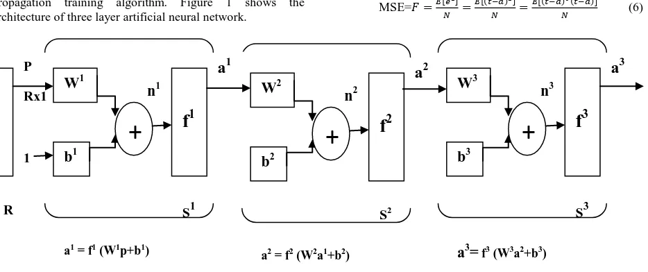
In this work, artificial neural network was used for implementing basic digital gates and image compression. The architecture of artificial neural network used in this research is a multi layer perceptron with steepest descent back propagation training algorithm. Figure 1 shows the architecture of three layer artificial neural network.

If the artificial neural network has M layers and receives input of vector p, then the output of the network can be calculated using the following equation:

₎

) _{) ) (1)}

Where, is the transfer function, and are weight and bias of the layer m. For m=1, 2 …M.

For three layer network shown in Fig 1, the output a3 is given as:

) ) ) (2)

The back propagation algorithm implemented here can be derived as follows [1] [6]:

The neurons in the first layer receive external inputs:

(3)

The above equation provides the starting point of the network. The outputs of the neurons in the last layer are considered the network outputs:

(4)

The performance index of the algorithm is the mean square error at the output layer. Since the algorithm is the supervised learning method, it is provided with set of examples of proper network behavior. This set is the training set for the neural network, for which the network will be trained as shown in equation below:

{ } { } { } (5)

Where, is an input vector to the network, and is the corresponding target output vector of the network. At each iteration, input is applied to the network and the output is

algorithm should adjust the network parameters i.e., weights and biases in order to minimize the mean square error (MSE) given below:

MSE= [ ] [ )] [ ) )] (6)

The back propagation algorithm calculates how the error depends on the output, inputs, and weights. After which the weights and biases are updated. The change in weight ) and bias ) is given by the equation 7 and 8 respectively.

) (7)

) (8)

Where, is the learning rate at which the weights and biases of the network are adjusted at iteration

The new weights and biases for each layer at iteration are given in equations 9 and 10 respectively.

) )

(9)

) ) (10)

So, we only need to find the derivative of w.r.t and . This is the goal of the back propagation algorithm, since we need to achieve this backwards. First, we need to calculate how much the error depends on the output. By using the concept of chain rule the derivative

and

can be

written as shown in the equation 11 and 12 respectively.

(11)

(12)

Where, ∑ (13)

Therefore,

(14)

a

n

W

b

f

+

S2

a2 = f2 (W2a1+b2) 1

P

Rx1

R

a

n

W

b

f

+

S1

a1 = f1 (W1p+b1)

a

n

W

b

f

+

S3

a

=

Now if we define

(15)

In matrix form the updated weight matrix and bias matrix at k+1th pass can be written as:

) ) ) (16) ) ) (17) Where , the sensitivity matrix is

(18)

Now it remains for us to compute the sensitivities , this requires another application of chain rule. It is this process that gives the term back propagation, because it describes a recurrence relationship in which the sensitivity at layer is computed from the sensitivity at layer . Therefore by applying chain rule to we get:

(19)

Then

can be simplified as

_{) (20)}

Where,

)

[

)

)

]

(21)

Now the sensitivity sm can be simplified as:

) ) (22)

We still have one more step to complete back propagation algorithm. We need to find out the starting point for the recurrence relation of the equation 22. This is obtained at the final layer:

) ) (23)

Since,

) ) (24)

So we can write

) ) (25)

The back propagation algorithm can be summarized as follows:

a. Initialize weights and biases to small random numbers.

b. Present a training data set to neural network and calculate the output by propagating the input forward through the network using network output equation.

c. Propagate the sensitivities backward through the network:

) )

) _{) For m=M-1...2, 1}

d. Calculate weight and bias updates and change the weights and biases as:

) ) ₎

) )

e. Repeat step 2 – 4 until error is zero or less than a limit value.

3.

TRAINING

NEURAL

NETWORK

USING

BACK

PROPAGATION

ALGORITHM TO IMPLEMENT BASIC

DIGITAL GATES

Basic logic gates form the core of all VLSI design. So, ANN architecture is trained on chip using back propagation algorithm to implement basic logic gates. In order to train on chip for a complex problem, image compression and decompression is selected. Image compression is selected on the basis that ANN are more efficient than traditional compression techniques like JPEG at higher compression ratio.

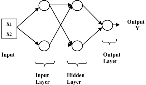
The Figure 2 shows the architecture of 2:2:2:1 neural network selected to implement basic digital gates i.e, AND, OR, NAND, NOR, XOR, XNOR function. The network has two inputs x1 and x2 with output y. In order to select the transfer funtion to train the network, MATLAB analysis is done on the neural network architecture and it is found that TANSIG (hyperbolic tangent sigmoid) transfer function gives the best convergence of error during the training to implement digital gates.

Figure 2: Structure of 2:2:2:1Neural Network X1

X2

Input s

Input Layer

Hidden Layer

Output Layer

3.1

Simulation Results

In order to implement the neural network along with the training algorithm on FPGA, the design is implemented using verilog and is simulated in MODELSIM. And the untrained network output obtained after simulation is erroneous but once the network is trained it is able to implement basic digital operations.

For FPGA implementation the simulated verilog model is synthesized in Xilinx ISE 10.1 and the net-list is obtained, which is mapped onto SPARTAN3 FPGA. The 2:2:2:1 network with training algorithm consumes 81% of the area on SPARTAN3 FPGA. The functionality of the training algorithm on FPGA to train 2:2:2:1 neural network is verified using XILINX CHIPSCOPE 10.1 tool.

4.

TRAINING

NEURAL

NETWORK

USING

BACK

PROPAGATION

ALGORITHM TO IMPLEMENT IMAGE

COMPRESSION

Artificial Neural Network (ANN) based techniques provide means for the compression of data at the transmitting side and decompression at the receiving side [7]. Not only can ANN based techniques provide sufficient compression rates of the data in question, but security is easily maintained [8]. This occurs because the compressed data that is sent along a communication channel is encoded and does not resemble its original form [9].

Artificial Neural Networks have been applied to many problems, and have demonstrated their superiority over classical methods when dealing with noisy or incomplete data. One such application is for data compression [7], [10]. Neural networks seem to be well suited to this particular function, as they have an ability to preprocess input patterns to produce simpler patterns with fewer components. This compressed information (stored in a hidden layer) preserves the full information obtained from the external environment. The compressed features may then exit the network into the external environment in their original uncompressed form.

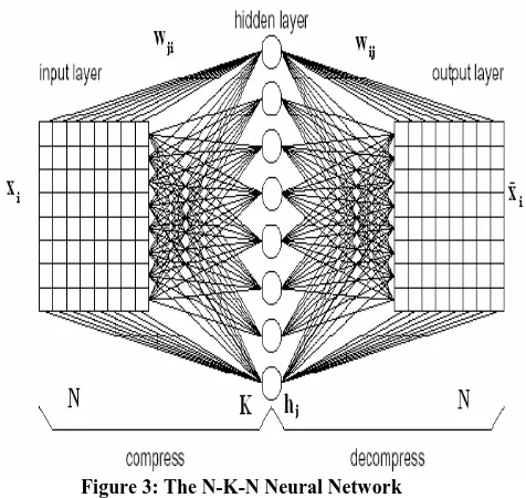
The network structure for image compression and decompression is illustrated in Figure 3[9]. This structure is referred to feed forward type network. The input layer and output layer are fully connected to the hidden layer. Compression is achieved by estimating the value of K, the number of neurons at the hidden layer less than that of neurons at both input and the output layers.

The data or image to be compressed passes through the input layer of the network, then subsequently through a very small number of hidden neurons. It is in the hidden layer that the compressed features of the image are stored, therefore the smaller the number of hidden neurons, the higher the compression ratio. The output layer subsequently outputs the decompressed image. It is expected that the input and output data are the same or very close. If the network is trained with appropriate performance goal, then the input image and output image are almost close.

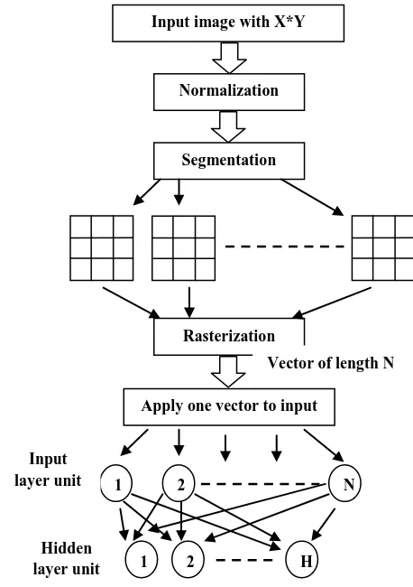
A neural network can be designed and trained for image compression and decompression. Before the image can be used as data for training the network or as input for compression, certain pre-processing should be done on the input image data. The pre-processing includes normalization, segmentation and rasterization [7] [11]. The pre-processed

image data can be either used for training the network or as input data for compression.

The input image is normalized with the maximum pixel value. The normalized pixel values for grey scale images with grey levels [0,255] in the range [0, 1]. The reason of using normalized pixel values is due to the fact that neural networks can operate more efficiently when both their inputs and outputs are limited to a range of [0,1].

Figure 3: The N-K-N Neural Network

This also avoids use of larger numbers in the working of the network, which reduces the hardware requirement drastically when implemented on FPGA.

If the image to be compressed is very large, this may sometimes cause difficulty in training, as the input to the network becomes very large. Therefore in the case of large images, they may be broken down into smaller, sub-images. Each sub-image may then be used to train an ANN or for compression. The input image is split up into blocks or vectors of 16x16, 8x8, 4x4 or 2x2 pixels. This process of splitting up the image into smaller sub-images is called segmentation [9]. Usually input image is split up into a number of blocks, each block has N pixels, which is equal to the number of input neurons.

Finally, since the sub-image is in 2D form, rasterization is done to convert it into 1D form i.e., vector of length N. The flow graph for image compression at the transmitter side is as shown in the Figure 4[11]. The similar inverse processes have to be done for decompression at the receiver side. Image compression is achieved by training the network in such a way that the coupling weights { wij }, scale the input vector of

N-dimension into a narrow channel of K-dimension (K<N) at the hidden layer and produce the optimum output value which makes the error between input and output minimum.

training algorithm with appropriate performance goal so the input image and output image are almost close.

The training is done for gray scale images of pixel size 256X256. The image is normalized first, then the large image is split up into sub-images of size 2X2 pixel i.e., segmentation and rasterization is done to convert 2X2 image pixels into a vector of 4 pixels. This vector forms the four inputs to the network. The same pre-processing is done on the training image and the vectors are stored on the FPGA, which are used while training the network

Figure 4: Flow Graph for Image Compression

Figure 5: A 4:4:2:2:4 Neural Network

For the selected 4:4:2:2:4 network, it is necessary to find the appropriate transfer function for the neurons for image compression. The transfer function is selected so that, when the network is trained there is error convergence and performance goal is met. In order to select the transfer function, MATLAB analysis is done for 4:4:2:2:4 network using various transfer functions like PURELIN, LOGSIG and TANSIG.

An image is selected for training which is shown in Figure 6a (LENA image). The network is trained in MATLAB with initial random weights, biases using the training image for various transfer functions and the network is tested using a test image which is shown in Figure 6b. The network is trained using MATLAB neural network toolbox back propagation training function “TRAINGD”.

(a) (b)

Figure 6 a: Training Image (LENA image) b: Test Image

X1 X2 X3 X4

Input s

Input Layer

Hidden Layers

Output Layer

Output Y1

Y2

Y3

Y4

Input image with X*Y

dimensions

Normalization

Segmentation

Rasterization

Apply one vector to input layer

1 2 N

1 2 H

Vector of length N

Input layer unit

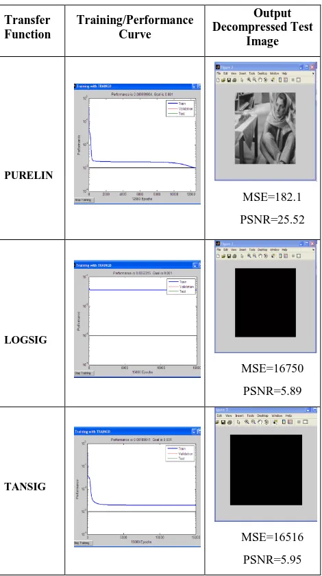
The results of the analysis are as shown in the Table 1. From the table we can conclude that, with only PURELIN transfer function, the network can be trained to meet the performance goal and the error converges. The MSE obtained using purelin transfer function is the least compared to other transfer function i.e., 182.1. Also the output decompressed test image is viewable only in the case of network with PURELIN transfer function. So we conclude that PURELIN transfer function is the better transfer function for training 4:4:2:2:4 neural network for image compression and decompression

Table 1: MATLAB 4:4:2:2:4 Analysis Results

Transfer Function

Training/Performance Curve

Output Decompressed Test

Image

PURELIN

MSE=182.1

PSNR=25.52

LOGSIG

MSE=16750

PSNR=5.89

TANSIG

MSE=16516

PSNR=5.95

The Back propagation training algorithm code for 4:4:2:2:4 neural network with PURELIN transfer function is implemented in MATLAB. The neural network is trained for image compression and decompression using back propagation algorithm. The coding is done with all the pre-processing on the input image. The same images as shown in figure 6 are used as training and test images respectively. The results from matlab implementation are as shown below in the Table 2 for untrained and trained network.

From the results of Table 2, it can be seen that the untrained network output image is fuzzy and not viewable. But the

be seen that the MSE of network output is almost same to that of MSE obtained in Table 1 for PURELIN transfer function. Therefore it can be concluded that the back propagation algorithm implemented in MATLAB is in terms with that of the MATLAB training function TRAINGD.

The general structure for 4:4:2:2:4 artificial neural network with online training is as shown in Figure 7. Since the training is done online i.e., on FPGA other than in system, the neural network will function in two modes: training mode and operational mode. When the ‘train’ signal is high the network is in training mode or else it will be in operational mode. The network is trained for image compression and decompression.

Table 2: 4:4:2:2:4 Network Matlab Implementation Output

Untrained Network Decompressed Output

Trained Network Decompressed Output

MSE=15625

PSNR=6.1926

MSE=177.4908

PSNR= 25.6390

Figure 7: 4:4:2:2:4 Network Structure

Verilog coding for the 4:4:2:2:4 neural network and back propagation training algorithm is done, so the network can be trained online for image compression and decompression. The verilog model is simulated in MODELSIM; the untrained network output pixel values are very far from input values and fuzzy. But once the network is trained, the output pixel values

4:4:2:2:4

Neural

Network

X1

X2

X3

X4

Train

Clock

Y1

Y2

Y3

network output for [255,255,255,255] input pixel set is [41,-126, 66,-21]. But trained network output set is [248,248,242,241].

The verilog model of 4:4:2:2:4 neural network with online training is synthesized in XILINX ISE 10.1 and implemented on VIRTEX 2pro FPGA. Device utilization summary for 4:4:2:2:4 neural network with online back propagation training is shown in the Table 3.

Table 3: Device Utilization Scheme of 4:4:2:2:4 Network

FPGA Device: VIRTEX 2pro Device name: 2vp30- ff896-7

Number of Slices 1847 out of 13696 13%

Number of Slice Flip

Flops 2121 out of 27392 7%

Number of 4 input LUTs 2709 out of 27392 9%

Number of IOs 70

Number of bonded IOBs 70 out of 556 12%

Number of MULT18X18s 116 out of 136 85%

Number of GCLKs 8 out of 16 50%

Number of BRAMs 36 out of 136 26%

The 4:4:2:2:4 neural network implemented on FPGA is verified using Xilinx Chipscope Pro Analyzer which is an on chip verification tool. The network is trained on-line on FPGA for image compression and decompression. The decompressed pixel output of untrained and trained network matches with the MODELSIM results.

5.

CONCLUSION AND FUTURE SCOPE

The back propagation algorithm for training multilayer artificial neural network is studied and successfully implemented on FPGA. This can help in achieving online training of neural networks on FPGA than training in computer system and make a trainable neural network chip. In terms of hardware efficiency, the design can be optimized to reduce the number of multipliers. The training time for the network to converge to the expected output can be reduced by implementing the adaptive learning rate back-propagation algorithm. By doing this there is an area tradeoff for speed. Also the timing performance of the network can be improved by designing a larger neural network with more number of neurons. This will allow the network to process more number of pixels and reduce the time of operation. With all the optimization and on-line training we would be able to build a more complex neural network chip, which can be trained for realizing complex functions.

6.

ACKNOWLEDGEMENTS

We would like to thank Nitte Meenakshi Institute of Technology for giving us the opportunity and facilities to carry out this work. We would also like to thank the faculty members of the Electronics and Communication Department for all their help and support. We also acknowledge that this research work is supported by VTU vide grant number VTU/Aca - RGS/2008-2009/7194.

7.

REFERENCES

[1] Martin T. Hagan, Howard B. Demuth, Mark Beale, “Neural Network Design”, China Machine Press, 2002.

[2] Himavathi, Anitha, Muthuramalingam, “Feed forward Neural Network Implementation in FPGA Using Layer Multiplexing for Effective Resource Utilization”, Neural Networks, IEEE Transactions-2007.

[3] Rafael Gadea, Franciso Ballester, Antonio Mocholí, Joaquín Cerdá, “Artificial neural network implementation on a single FPGA of a pipelined on-line backpropagation” ISSS Proceedings of the 13th international symposium on System synthesis, IEEE Computer Society 2000.

[4] M. Hajek, “Neural Networks”, 2005.

[5] R. Rojas, “Neural Networks”, Springer-Verlag, Berlin, 1996,.

[6] Thiang, Handry Khoswanto, Rendy Pangaldus, “Artificial Neural Network with Steepest Descent Backpropagation Training Algorithm for Modeling Inverse Kinematics of Manipulator”, World Academy of Sciences, Engineering and Technology, 2009.

[7] B. Verma, M. Blumenstein and S. Kulkarni, “A Neural Network based Technique for Data Compression”, Griffith University, Gold Coast Campus, Australia.

[8] Venkata Rama Prasad Vaddella, Kurupati Rama, “Artificial Neural Networks For Compression Of Digital Images: A Review”, International Journal of Reviews in Computing, 2009-2010.

[9] Rafid Ahmed Khalil, “Digital Image Compression Enhancement Using Bipolar Backpropagation Neural Networks”, University of Mosul, Iraq, 2006.

[10] S. Anna Durai, and E. Anna Saro,”Image Compression with Back Propagation Neural Network using Cumulative Distribution Function” World Academy of Sciences, Engineering and Technology, 2006.