Factor Vector Autoregressive Estimation of Heteroskedastic Persistent and Non Persistent Processes Subject to Structural Breaks

(1)

http://dx.doi.org/10.4236/ojs.2014.44030

How to cite this paper: Morana, C. (2014) Factor Vector Autoregressive Estimation of Heteroskedastic Persistent and Non Persistent Processes Subject to Structural Breaks. Open Journal of Statistics, 4, 292-312.

http://dx.doi.org/10.4236/ojs.2014.44030

Factor Vector Autoregressive Estimation

of Heteroskedastic Persistent and Non

Persistent Processes Subject to

Structural Breaks

Claudio Morana

1,2

1_{Department of Economics, Management and Statistics, University of Milan-Bicocca, Milan, Italy} 2_{Center for Research on Pensions and Welfare Policies, Collegio Carlo Alberto, Moncalieri, Italy} Email: [email protected]

Received 22 March 2014; revised 18 April 2014; accepted 6 May 2014

This work is licensed under the Creative Commons Attribution International License (CC BY). http://creativecommons.org/licenses/by/4.0/

Abstract

In the paper, a general framework for large scale modeling of macroeconomic and financial time series is introduced. The proposed approach is characterized by simplicity of implementation, performing well independently of persistence and heteroskedasticity properties, accounting for common deterministic and stochastic factors. Monte Carlo results strongly support the proposed methodology, validating its use also for relatively small cross-sectional and temporal samples.

Keywords

Long and Short Memory, Structural Breaks, Common Factors, Principal Components Analysis, Fractionally Integrated Heteroskedastic Factor Vector Autoregressive Model

1. Introduction

In the paper, a general strategy for large-scale modeling of macroeconomic and financial data, set within the factor vector autoregressive model (F-VAR) framework, is proposed.1

Following the lead of dynamic factor model analysis proposed in [2], it is assumed that a small number of structural shocks are responsible for the observed comovement in economic data; it is, however, also assumed that commonalities across series are described by deterministic factors, i.e., common break processes. Comove- ment across series is then accounted by both deterministic and stochastic factors; moreover, common factors are

(2)

293

allowed in both mean and variance, covering the I(0) and I(1) persistence cases, as well as the intermediate case of long memory, i.e., I(d), 0< <d 1. As the common factors are unobserved, accurate estimation may fail in the framework of small scale vector autoregressive (VAR) models, but succeed when cross-sectional information is employed to disentangle common and idiosyncratic features.

The proposed fractionally integrated heteroskedastic factor vector autoregressive model (FI-HF-VAR) bridges the F-VAR and (the most recent) G-VAR literature, as, similarly to [3], a weakly stationary cyclical representation is employed; yet, similarly to [4], principal components analysis (PCA) is employed for the estimation of the latent factors. Consistent and asymptotically normal estimation is performed by means of QML, also implemented through an iterative multi-step estimation procedure. Monte Carlo results strongly support the proposed methodology.

Overall, the FI-HF-VAR model can be understood as a unified framework for large-scale econometric modeling, allowing for accurate investigation of cross-sectional and time series features, independent of persistence and heteroskedasticity properties of the data, from comovement to impulse responses, forecast error variance and historical decomposition analysis.

After this introduction, the paper is organized as follows. In Section 2, the econometric model is presented; in Section 3, estimation is discussed, while Monte Carlo analysis is performed in Section 4; finally, conclusions are drawn in Section 5.

2. The FI-HF-VAR Model

Consider the following fractionally integrated heteroskedastic factor vector autoregressive (FI-HF-VAR) model

( )

(

1 1 1

)

Λ Λ Λ Λ

t t f t t t f t t

x − µµ − f =C L x− − µµ− − f− +v (1)

(

)

. . . 0,

t v

v ∼i i d Σ

( ) ( )

1/ 2

t t t t

P L D L f =

η

=H

ψ

(2)

(

)

. . . 0,

t i i d IR

ψ

∼

where x_t is a N×1 vector of real valued integrated I(d) ( 0≤ ≤d 1) and heteroskedastic processes subject to structural breaks, t=1,, ,T in deviation from the unobserved common deterministic (µ_t) and stochastic (ft)

factors;

( )

0 0 1 2 2

s s

C L ≡C L +C L C L+ + + C L is a finite order matrix of polynomials in the lag operator with

all the roots outside the unit circle, C_j, j=0,,s, is a square matrix of coefficients of order N; v_t is a 1

N× vector of zero mean idiosyncratic i.i.d. shocks, with contemporaneous covariance matrix Σ_v, assumed to be coherent with the condition of weak cross-sectional correlation of the idiosyncratic components (Assumption E) stated in [5] p. 143. The model in (1) actually admits the same static representation of [5], as it can be rewritten as xt Λ_μ

µ

t Λf ft

(

I C L

( )

)

1vt

−

= + + − .

2.1. The Common Break Process Component

The vector of common break processes µ_t is M×1, with M ≤N , and N M× matrix of loadings Λ_µ; the

latter are assumed to be orthogonal to the common stochastic factors f_t, and of unknown form, measuring recurrent or non recurrent changes in mean, with smooth or abrupt transition across regimes; the generic element in 𝜇𝜇_𝑡𝑡is 𝜇𝜇_𝑖𝑖_,_𝑡𝑡 ≡ 𝑧𝑧_𝜇𝜇_,_𝑖𝑖(𝑡𝑡), where zµ_,i

( )

t ,i=1,,M, is a function of the time index t, t=1,,T.

The idiosyncratic break process zµ,i

( )

t can take different forms. For instance, [6] use a discontinuous function,

( )

, ,0 1 , j,

J

i i j i j

z_µ t =

δ

+

∑

₌

δ

I_τ (3)

where

j

I_τ is the indicator function, such that 1

j

I_τ = if t>τ_j and is 0 otherwise; in [6] the break points τ_j

(3)

294 this purpose.

Differently, [8] [9] and [10] model the break process as a continuous and bounded function of time, by means of a Fourier expansion, i.e.,

( )

(

)

(

)

, ,0 1 , , sin 2 , , cos 2 ,

2 J

i i j i s j i c j

T

z_µ t =δ +

∑

₌δ πjt T +δ π jt T j≤ (4)

Similarly [11], using a logistic specification

( )

(

*

)

, ,0 1 , , , ,

J

i i j i j j j

z_µ t =

δ

+

∑

₌

δ

g

η

c t (5)

where the logistic function is

(

)

(

( )

(

)

*

)

1

* * _ˆ

, , 1 exp

j j j _t

g η c t γ η t c σ

−

= + − − , γ η

( )

=exp

( )

ηj , cj∈

[ ]

0,1 and

j

η are parameters, t*=t T , and

σ

ˆ_t* is the estimated standard deviation of

*

t . In particular, as η_j → ∞,

( )

g ⋅ becomes the indicator function, yielding therefore a generalization of the specification in [6]. Also similarly [12] and [13], using a spline function

( )

,i

zµ t =S t T , (6)

where

( )

2

( )

1 p

j j j

S t T =

∑

₌+ a f t T is a spline function of order p, a_j are unknown regression coefficients and

the functions f_j

( )

⋅ are spline basis functions defined as f₁=1, f₂=

( )

t T ,, f_p+₁=

( )

t T p, and

(

)

2

p p

f ₊ = t T−η , with

η

∈

(

1T,1

)

.

A semiparametric approach has also been suggested by [14], using a kernel function, i.e.,

( )

, 1 ,

1 T j

i j i j

t t

z t K x

Tb b

µ =

−

 

= _ _

 

∑

, (7)

where b is the bandwidth and K

( )

⋅ is the kernel function, specified as K u

( )

=

∑

_lr₌₀α_lu2l for u ≤1 and

( )

0

K u = for u >1; r=0,1, 2,, and the coefficient α_l are such that 1

( )

1K u du 1

− =

∫

.

Finally, a random level shift model has been proposed by [15]-[18]; for instance, [18] define the break process as

( )

, 1 , , ,

T

i j T i j

z_µ t =

∑

₌

δ

(8)

where δ_{T i j}_{, ,} =π_{T t}_,η η_t, _t ~ . . .i i d N

(

0,σ2

)

and π ~ . . .T t, i i d Bernoulli p T

(

,1

)

for p≥0.

In the case M =N , there are no common break processes, i.e., each series is characterized by its own idiosyncratic break process and the N M× factor loading matrix Λ_µ is square, diagonal and of full rank; when

M <N , there exist M common break processes and the factor loading matrix is of reduced rank (M). Hence, in the latter case the series x_t are cotrending, according to [19], nonlinear cotrending, according to [20], or cobreaking, according to [21] and [22]. The representation in (1) emphasizes however the driving role of the common break processes, rather than the break-free linear combinations (cobreaking/cotrending relationships) relating the series x_t.

2.2. The Common Break-Free Component

The vector of (zero-mean) integrated heteroskedastic common factors f_t is R×1, with R≤N, and N×R

matrix of loadings Λ_f . The order of integration is d_i in mean, and b_i in variance, 0≤di ≤1, 0≤ ≤bi 1, 1, ,

i=  R.

The polynomial matrix

( )

1 2 2

u

R u

P L ≡I −P L−P L − − P L is of finite order, with all the roots outside the unit

(4)

295

The matrix D L

( )

is a square diagonal matrix in the lag operator of order R, specified according to the integration order (in mean) of the common stochastic factors, i.e., D L

( ) (

≡ −1 L I

)

_R for the case of I

( )

1 integration (di =1);D L

( )

≡IR for the I

( )

0 or no integration (short memory) case (di =0);

( )

{

(

) (

1

)

2

(

)

}

1 d , 1 d , , 1 dR

D L ≡diag −L −L  −L for the case of fractional integration (I d

( )

, long memory)

(0<di<1), where

(

1

)

i

d

L

− is the fractional differencing operator; the latter admits a binomial expansion, which can be compactly written in terms of the Hypergeometric function, i.e.,

(

)

(

)

(

) (

) ( )

1 1

0 0

1 di ,1,1; Γ Γ 1 Γ k π k

i k i i k k

L F d L ∞₌ k d k − d − L ∞₌ L

− = − ≡

∑

− + − ≡

∑

, where Γ

( )

⋅ is the Gamma func-

tion.

In the case R=N there are no common stochastic processes, i.e., each series is characterized by its own idiosyncratic persistent stochastic component, and the N×R factor loading matrix Λ_f is square, diagonal and of full rank; when R<N, then there exist R common stochastic processes and the factor loading matrix is of reduced rank (R). Hence, in the latter case the series x_t show common stochastic features, according to [23]. The concept of common feature is broad, encompassing the notion of cointegration ([24]), holding for the

0<di≤1 case. The representation in (1) emphasizes however the driving role of the common stochastic fac-tors rather than the feature-free linear combinations (cofeature relationships) relating the series x_t.

2.3. The Conditional Variance Process

The R R× conditional variance-covariance matrix for the unconditionally and conditionally orthogonal com-

mon factors f_t is Ht=Var f

(

t Ωt−₁

)

≡diag h

{

_1,t,h_2,t,,hR t_,

}

, where Ωt−1 is the information set available at

time period t−1. Consistent with the constant conditional correlation model of [25], the ith generic element along the main diagonal of H_t is

( )

2

, , , , 1, , ,

i i t i t i i t

m L h =

ω

+n L

η

i=  R (9)

where

( )

1

( )

(

1

( )

)

(

1

)

bi

i i i

n L ≡ −β L − −ϕ L −L for the case of fractional integration (long memory) in variance

(0< <bi 1); n Li

( )

≡ −1 βi

( )

L − −

(

1 ϕi

( )

L

)

(

1−L

)

for the case of I

( )

1 integration in variance (bi =1);

( )

1

( )

(

1

( )

)

i i i

n L ≡ −β L − −ϕ L for the I

( )

0 or no integration (short memory) in variance case (bi=0). In all

casesm L

( )

≡ −1

β

i

( )

L ,

ϕ

i

( )

L =

α

i

( )

L +

β

i

( )

L ,

( )

2

,1 ,2 ,

q

i L i L i L i qL

α

≡

α

+

α

+ +_

α

,

( )

2

,1 ,2 ,

p

i L i L i L i pL

β

≡

β

+

β

+ +_

β

and all the roots of the

α

_i

( )

L and

β

_i

( )

L polynomials are outside the unit circle.

The conditional variance process h_{i t}_, =Var f

(

_{i t}_, Ω_{i t}_,−₁

)

, i=1,,R, is therefore of the FIGARCH p b z

(

, ,i

)

type [26], with z=max

{ }

p q, , or the IGARCH p q

(

,

)

type, for the fractionally integrated and integrated case, respectively; of the GARCH p q

(

,

)

type for the non integrated case. The model is however not standard

as the intercept component ω_{i t}_, is time-varying, allowing for structural breaks in variance; similarly to the mean part of the model, structural breaks in variance are assumed to be of unknown form, measuring recurrent or non recurrent regimes, with smooth or abrupt transition; then,

ω

_{i t}_, ≡z_{h i}_,

( )

t , where z_{h i}_,

( )

t is a continuos or

discontinuous bounded function of the time index t, t=1,,T, which can be parameterized as in (3), (4), (5), (6), (7), or (8).

The following ARCH (∞) representation can be obtained from each of the three above models

( )

* 2

, , , 1, , ,

i t i t i i t

h =

ω

+

ψ

L

η

i=  R (10)

where

( )

, *

,

1 i t i t

i

m

ω

ω = and

( )

1, 2, 2

i

i i i

i

n L

L L L

m L

ψ = =ψ +ψ +_.

(5)

296

riance process (no integration case), or long-term conditional variance level (unit root and fractional integration cases).

To guarantee the non negativity of the conditional variance process at eachpoint in time all the coefficients in the ARCH

( )

∞ representation must be non-negative, i.e., ψi j_, ≥0 for all j≥1 and

*

, 0

i t

ω

> for any t. Sufficient conditions, for various parameterization, can be found in [26] and [27].

2.4. The Reduced Fractional VAR form

By substituting (2) into (1) and rearranging, the vector autoregressive representation for the factors f_t and the gap series x_t−Λµµ_t can be written as

( )

* 1 * 1 1 0 Λ Λ

t f t t

t t t t t

f L f

x µµ L C L x µµ ε

η − − −         =_ _ +  ₋   ₋            Π Π

  (11)

1/ 2 0

, Λ t t t f t t I H v

η

ψ

ε

   ₌ _ _₊               

where *

( )

L Λf

( )

L L1 C L

( )

Λf −

 

=_ −

Π _ and Πf*

( )

L is differently defined according to persistence properties of the data. In particular, for the case of fractional integration (long memory)

(

0<di<1

)

, by means of the

binomial expansion, it follows P L D L

( ) ( )

≡ − ΠI

( )

L , Π

( )

L = Π + Π₁L ₂L2+, where Π_i, i=1, 2,, is a square matrix of coefficients of dimension R, and Π_f*

( )

L = Π

( )

L L−1; since the infinite order representation

cannot be handled in estimation, a truncation to a suitable large lag for the polynomial matrix Π

( )

L is re-

quired.2 Hence,

( )

* 1

p j

j j

L ₌ L

Π ≅

∑

Π . For the case of no integration (short memory) (di =0), recalling

that D L

( )

≡I_R, and therefore P L D L

( ) ( )

=P L

( )

, then Π

( )

L = Π + Π₁L ₂L2+ + Π _uLu; for the case of inte-

gration (di =1), it should be firstly recalled that

( ) ( )

( )(

) (

)

(

2

)

(

)

1 2

1 R u u 1

P L D L ≡P L −L ≡ I −ρL − P L+P L + + P L −L , with ρ =I_R; the latter may be rewrit-

ten in the equivalent polynomial matrix form I_R− Γ − Γ₁L ₂L2− − Γ _u+₁Lu+1, where Γi, i=1,,u+1, is a square matrix of coefficients of dimension R, and Γ₁+ Γ + + Γ₂ ... u+₁= =

ρ

IR,Pi= −

(

Γi+₁+ Γ + + Γi+₂ ... u+₁

)

,

1, 2, ,

i=  u; then, Π

( )

L =P L₁ +P L₂ 2+ +... P Lu u.

Reduced Form and Structural Vector Moving Average Representation of the FI-HF-VAR Model

In the presence of unconditional heteroskedasticity, the computation of the impulse response functions and the forecast error variance decomposition (FEVD) should be made dependent on the estimated unconditional variance for each regime. In the case of (continuously) time-varying unconditional variance, policy analysis may then be computed at each point in time. For some of the conditional variance models considered in the paper, i.e., the FIGARCH and IGARCH processes, the population unconditional variance does not actually exist; in the latter cases the ω_{i t}_, component might bear the interpretation of long term level for the conditional variance; policy analysis is still feasible, yet subject to a different interpretation, FEVD referring, for instance, not to the proportion of forecast error (unconditional) variance accounted by each structural shock, but to the proportion of forecast error (conditional) long term variance accounted by each structural shock. With this caveat in mind, the actual computation of the above quantities is achieved in the same way as in the case of well defined population unconditional variance.

Hence, the computation of the vector moving average (VMA) representation for the FI-HF-VAR model de-

2

(6)

297

pends on the persistence properties of the data. The following distinctions should then be made.

For the short memory case, i.e., the zero integration order case

(

d_i =0

)

, the VMA representation for the factors f_t and gap series x_t−Λµµ_t can be written as

( )

0 Λ

t t

t t t

f U L

x µ

µ

G L F L v

η

      =    ₋     

    , (12)

where U L

( )

≡P L

( )

−1, G L

( )

≡Λ_fP L

( )

−1 and F L

( )

≡_I−C L L

( )

_−1.

For the long memory case (0<di<1) and the case of I

( )

1 non stationarity (di =1), the VMA representation should be computed for the differenced process, yielding

(

)

( )

0 1 Λ t t

t t t

f U L

L

x _µµ _{G L} _{F L} v

η + + +     _ _  − _ _= _{ } − _ _{  }

 _{ } _ , (13)

where U L

( ) (

+≡ −1 L U L

) ( )

, G L

( ) (

+ ≡ −1 L G L

) ( )

and F L

( ) (

+ ≡ −1 L F L

) ( )

. Impulse responses can

then be computed as

1 k

j j

I+

∑

₌U+ for f_t and

1 k

j j

I+

∑

₌G+ and

1 k

j j

I+

∑

₌ F+ for x_t−Λµµ_t, k=1, 2,

The identification of the structural shocks in the FI-HF-VAR model can be implemented in two steps. Firstly, denoting by ξ_t the vector of the R structural common factor shocks, the relation between reduced and structural form common shocks can be written as ξ_t =Hη_t, where H is square and invertible. Therefore, the identification of the structural common factor shocks amounts to the estimation of the elements of the H matrix. It is assumed that E

[ ]

ξ ξ

t t′ =IR, and hence HΣηH′ =IR. As the number of free parameters in Ση is

(

1 2

)

R R+ , at most R R

(

+1 2

)

parameters in H−1 can be uniquely identified through the Ση =H H−1 ′−1

system of nonlinear equations in the unknown parameters of H−1. Additional R R

(

−1 2

)

restrictions need

then to be imposed for exact identification of H−1, by constraining the contemporaneous or long-run responses to structural shocks; for instance, recursive (Choleski) or non recursive structures can be imposed on the VAR model for the common factors through exclusion or linear/non-liner restrictions, as well as sign restrictions, on the contemporaneous impact matrix H−1.3

Secondly, by denoting _t the vector of N structural idiosyncratic disturbances, the relation between reduced form and structural form idiosyncratic shocks can be written as _t =Kv_t, where K is square and invertible. Hence, the identification of the structural idiosyncratic shocks amounts to the estimation of the elements of the

K matrix. It is assumed that E KK

[

'

]

=IN, and hence KΣ ′ =vK IN. Then, in addition to the N N

(

+1 2

)

equa-

tions provided by Σ_v =K K−1 ′−1, N N

(

−1 2

)

restrictions need to be imposed for exact identification of K−1,

similarly to what required for the common structural shocks.

Note that preliminary to the estimation of the Σ_v matrix, vˆ_t should be obtained from the residuals of an OLS regression of εˆ_t on ηˆ_t; the latter operation would grant orthogonality between common and idiosyncratic residuals.

The structural VMA representation can then be written as

( )

* * * 0 Λ t t

t t t

f U L

x µ G L F L

ξ µ       =    ₋       

     , (14)

where U*

( )

L =U L H

( )

−1, G*

( )

L =G L H

( )

−1, F*

( )

L =F L K

( )

−1, or

(

)

( )

* * * 0 1 Λ t t

t t t

f U L

L

x _µµ _G _L _F _L

ξ + + +         − _ _= _{ } − _ _{  }

 _{ } _  , (15)

where U*

( )

L + =U L

( )

+H−1, G*

( )

L + =G L

( )

+H−1, F*

( )

L +=F L

( )

+K−1, according to persistence proper-

ties, and Ei t_, ,ξ ′j t_,  = 0 any i j, .

(7)

298

3. Estimation

Estimation of the model can be implemented following a multi-step procedure, consisting of persistence analysis,

QML estimation of the common factors and VAR parameters in (1), QML estimation of the conditional mean model in (2) and the reduced form model in (11), QML estimation of the conditional variance covariance matrix in (2).

3.1. Step 1: Persistence Analysis

Each component x_{i t}_, , i=1,,N, in the vector time series x_t is firstly decomposed into its purely deterministic (trend/break process; b_{i t}_, ) and purely stochastic (break-free, l_{i t}_, =x_{i t}_, ,−b_{i t}_, ) parts.

It is then assumed that the data obey the model

, , ,, 1, , 1, ,

i t i t i t

x =b +l t=  T i=  N , (16)

where b_{i t}_, and l_{i t}_, are orthogonal, bi t, ≡zb i,

( )

t , with zb i,

( )

t a bounded function of the time index t, evolv- ing according to discontinuous changes (step function) or showing smooth transitions across regimes.

Depending on the specification of z_{b i}_,

( )

t , a joint estimate of the two components can be obtained following [7] [10] [11] [13] [14] [30], by setting up an augmented fractionally integrated ARIMA model

( )(

1

) (

(

1

)

, ,

)

,

i

d k

i t i t i t

L L L x b v

φ − − − = , (17)

where k=

{ }

0,1 is the integer differencing parameter, d_i is the fractional differencing parameter

(−0.5<di<0.5),

φ

( )

L is a stationary polynomial in the lag operator and vi t, is a white noise disturbance.

Heteroskedastic innovations can also be considered, by specifying v_{i t}_, ≡σ_{it t}e, with et ~ . . . 0,1i i d

( )

and the conditional variance process

σ

_it2 according to a model of the GARCH family.

Consistent and asymptotically normal estimation by means of QML, also implemented through iterative algo- rithms, is discussed in [10] [13] [14] [18] [31]. Extensions of the Markov switching [7], logistic [11] and random level shift [15]-[18] models to the long memory case have also been contributed by [32] [33] and [34], respectively.

Alternatively, following [6], a two-step procedure can be implemented: firstly, structural break tests are carried out and break points estimated; then, dummy variables are constructed according to their dating and the break process is estimated by running an OLS regression of the actual series x_{i t}_, on the latter dummies, as in (3); this yields bˆi t, computed as the fitted process and the stochastic part as the estimated residual, i.e., lˆi t, =xi t,,−bˆi t, ;

, ˆ

i t

b and lˆ_{i t}_, are then orthogonal by construction.4

As neglected structural breaks may lead to processes which appear to show persistence of the long memory or unit root type, as well as spurious breaks may be detected in the data when persistence in the error component is neglected, testing procedures robust to persistence properties are clearly desirable. In this respect, the RSS-based testing framework in [6] yields consistent detection of multiple breaks at unknown dates for I

( )

0 processes, as well as under long range dependence [35];5 moreover, under long range dependence, the validity of an estimated break process (obtained, for instance, by means of [6]) may also be assessed by testing the null hypothesis of long memory in the estimated break-free series (lˆ_{i t}_, ), as antipersistence is expected from the removal of a spurious break process [36] [37]. Structural break tests valid for both I

( )

0 and I

( )

1 series have also recently contributed in the literature.

3.2. Step 2: Estimation of the Conditional Mean Model

QML estimation of the reduced form model in (11) is performed by first estimating the latent factors and VAR

4_{The orthogonality of}

,

ˆ

i t

b and lˆi t, can however also be imposed when jointly estimating the deterministic and stochastic components by

means of augmented ARFIMA models.

5

(8)

299

parameters in (1); then, by estimating the conditional mean process in (2); finally, by substituting (2) into (1) in order to obtain a restricted estimate of the polynomial matrix Π*

( )

L .

3.2.1. Estimation of the Common Factors and VAR Parameters

Estimation of the common factors is performed by QML, writing the (misspecified) approximating model as

Λ Λ

t t f t t

x − µµ − f =v (18)

(

2

)

~ . . . 0,

t N

v i i d N σ I

(

2

)

~ . . . 0,

t R

f i i d N σ I

with log-likelihood function given by

( )

2

(

) (

)

2 1

Λ Λ Λ Λ

1 ln 2π – ln

2 2 2

t t f t t t f t

T

N t

x f x f

NT T

l

σ

I µ

µ

σ

=

′

− − − −

⋅ = − −

∑

. (19)

QML estimation of the latent factors and their loadings then requires the minimization of the objective function

(

) (

)

1 Λ Λ Λ Λ

T

t t f t t t f t

t= x µµ f x µµ f

′

− − − −

∑

(20)

which can be rewritten as

(

) (

)

(

) (

)

1 1

Λ Λ Λ Λ

T T

t t t t t f t t f t

t b b t l f l f

NT = µµ µµ NT =

′ ′

− − + − −

∑

, (21)

where x_t = +l_t b_t, as l_t and b_t are orthogonal vectors, as well as µ_t and f_t.

The solution to the minimization problem, subject to the constraints N−1Λ Λ′_µ _µ =I_M and N−1Λ′ Λ =_f _f I_R, is

given by firstly minimizing with respect to µ_t and f_t, given Λ_µ and Λ_f, yielding

(

)

(

1

)

(

)

1

ˆ_t Λ Λ Λµ µ µ Λ Λµ µ Λµb_t

µ ′ − = ′ − ′

(

)

(

1

)

(

)

1

ˆ _{Λ Λ Λ} _{Λ Λ} _Λ

t f f f f f f t

f ′ − = ′ − ′l

and then concentrating the objective function to obtain

(

)

(

1

)

(

)

1

)

1 1

Λ Λ Λ Λ Λ Λ Λ Λ

T T

t N t t N f f f f t

t b I b t l I l

T µ µ µ µ T

− −

= ′ − ′ + = ′ − ′

∑

, (22)

which can be mimized with respect to Λ_µ and Λ_f. This is equivalent to maximizing

(

)

1/ 2

(

)

1/ 2

(

)

1/ 2 '

(

)

1/ 2

1 1

Λ Λ Λ T Λ Λ Λ Λ Λ Λ T Λ Λ Λ

t t f f f t t f f f

t t

tr b b tr l l

T T

µ µ µ µ µ µ

′ − −

− −

= =

 _′ _′  _′ _′ ₊  _′ _′  _′ _′ 

 _ _   _ _ 



∑

 

∑

, (23)

which in turn is equivalent to maximizing

Λ ˆ Λ b

µΣ µ (24)

subject to N−1Λ Λ′_µ _µ =I_M, and

Λ ˆ Λ

fΣl f (25)

subject to N−1Λ Λ′_f _f =I_R.

The solution is then found by setting:

 _Λˆ

µ equal to the scaled eigenvectors of Σˆb, i.e., the sample variance covariance matrix of the break processes b_t, associated with its M largest eigenvalues; this yields

µ

ˆ_t=N−1Λˆµ′b_t, i.e., the scaled first M

(9)

300

 _Λˆ

f equal to the scaled eigenvectors of Σˆl, i.e., the sample variance covariance matrix of the break-free processes l_t, corresponding to its R largest eigenvalues; this yields f_t′=N−1Λˆ′_{f t}l , i.e., the scaled first R

principal components of l_t.

Note that PCA uniquely estimates the space spanned by the unobserved factors; hence, Λ_f and f_t (Λ_µ

and µ_t) are not separately identified, as the common factors f_t

( )

µ

_t and factor loading matrix Λ Λ_f

( )

_µ are

uniquely estimated up to a suitable invertible rotation matrix Hf

( )

Hµ , i.e., PCA delivers estimates of

(

)

*,t f t *,t t

f ≡H f µ ≡H_µµ and Λ_f_*≡Λ_fH−_f1

(

Λ_µ_*≡Λ_µH_µ−1

)

, and therefore a unique estimate of the common

components Λ_f f_t ≡Λ_f_{* *,}f _t

(

Λµµ_t≡Λµ_*µ_*,_t

)

only, which is however all what is required for the computation

of the gap vector.

As shown by [38], exact identification of the common factors can also be implemented, by appropriately con-straining the factor loading matrix while performing PCA or after estimation. In particular, three identification structures are discussed, involving a block diagonal factor loading matrix, yield by a statistical restriction imposed in estimation, and two rotation strategies, yielding a lower triangular factor loading matrix in the former case and a two-block partitioned factor loading matrix in the latter case, with identity matrix in the upper block and an un-restricted structure in the lower block.

Moreover, the number of common factors

(

R M,

)

is unknown and needs to be determined; several criteria are available in the literature, ranging from heuristic or statistical eigenvalue-based approaches [39] [40] to the more recent information criteria [41] and “primitive” shock ([42]) based procedures.

Finally, in order to enforce orthogonality between the estimated common break processes

( )

µˆ_*,_t and stochastic factors

( )

fˆ_*,_t , the above procedure may be modified by computing the stochastic component lˆ_t as the residuals from the OLS regression of x_{i t}_, on µˆ_*,_t; then PCA is implemented on (the break-free residuals) lˆ_t to yield fˆ_*,_t.

Estimation of the VAR parameters. Conditional on the estimated (rotated) latent factors, the polynomial matrix C L

( )

and the Λf* ΛfHf1

−

≡ and Λµ* ΛµHµ1 −

≡ (rotated) factor loading matrices are obtained by means of OLS estimation of the equation system in (1). This can be obtained by first (OLS) regressing the actual series

xt on the estimated common break processes

( )

µˆ*,t and stochastic factors

( )

fˆ*,t to obtain Λˆµ* and Λˆf*;

alternatively, Λˆµ* and Λˆf* can be estimated as yield by PCA, i.e., from the scaled eigenvectors of the matrices Σˆ_b and Σˆ_l, respectively; then, the gap vector is computed as x_t −Λˆ_µ_*

µ

ˆ_*,_t −Λˆ_f_{* *,}fˆ _t, as Λˆ_f fˆ_t =Λˆ_f_{* *,}fˆ_t and

* *,

ˆ _ˆ ˆ _ˆ

Λµ

µ

t=Λµ

µ

t, and C Lˆ

( )

is obtained by means of OLS estimation of the VAR model in (1).

3.2.2. Iterative Estimation of the Common Factors and VAR Parameters

The above estimation strategy may be embedded within an iterative procedure, yielding a (relatively more effi- cient) estimate of the latent factors and the VAR parameters in the equation system in (1).

The objective function to be minimized is then written as

( )

(

)

1

Λ , ,Λ , , T

t f t t t t

S f C L v v

NT

µ µ =

∑

₌ ′ (26)

where v_t =

(

I_N−C L L

( )

)(

x_t−Λµµ_t−Λ_f f_t

)

.

 Initialization. The iterative estimation procedure requires an initial estimate of the common deterministic

( )

µ

t and stochastic

( )

ft factors and the C L

( )

polynomial matrix, i.e., an initial estimate of the equation system in (1). The latter can be obtained as described in Section 3.2.1.

 Updating. An updated estimate of the equation system in (1) is obtained as follows.

° First, a new estimate of the M (rotated) common deterministic factors, and their factor loading matrix, is obtained by the application of PCA to the (new) stochastic factor-free series

( )

(

)

* *,ˆ 1 * *,ˆ 1 * *, 1

ˆ ˆ ˆ _ˆ

Λ Λ Λ

t f t t f t t

x − f −C L x− − f − − _µ

µ

− , yielding Λˆ(* ) new

µ and ˆ*,( ) new

t

µ .6

6_{Alternatively,} ( )

*

ˆ Λnew

µ can be obtained by regressing xt on

( )

*,

ˆnew t

(10)

301

° Next, conditional on the new common break processes and their factor loading matrix, the new estimate of the common long memory factors is obtained from the application of PCA to (new) break-free processes

( ) ( ) ( )

* *, ˆ

ˆnew _Λnew _ˆnew

t xt t

l = − _µ µ 7 yielding Λˆ(_fnew_* ) and fˆ_*,(_tnew).8

° Finally, conditional on the new estimated common break processes and long memory factors, the new estimate of the gap vector x_t−Λˆ(µnew_* ) (µˆ_*,new_t )−Λˆ(_fnew_* ) (fˆ_*,new_t ) is obtained, and the new estimate ˆ

( )

new

C L can be computed by means of OLS estimation of the VAR model in (1).

° The above procedure is iterated until convergence, yielding the final estimates Λˆ( )_µfin_* ,µˆ_*,( )fin_t , Λˆ( )_ffin_* ,fˆ_*,( )_tfin ,

and C Lˆ

( )

( )fin . Convergence may be assessed in various ways. For instance, the procedure may be stopped

when the change in the value of the objective function is below a given threshold.9

3.2.3. Restricted Estimation of the Reduced Form Model

Once the final estimate of the equation system in (1) is available, the reduced VAR form in (11) is estimated as follows:

1) For the case of fractional integration (long memory) (0<di <1), the fractional differencing parameter is

(consistently) estimated first, for each component of the (rotated) common factors vector fˆ_*,( )_tfin , yielding the es-

timates dˆ_i, i=1,,R, collected in D Lˆ

( )

matrix.

Considering then the generic element fˆ_*,( )_tfin, T consistent and asymptotically normal estimation of the ith

fractional differencing parameter can be obtained, for instance, by means of QML estimation of the fractionally integrated ARIMA model in (17); alternatively, consistent and asymptotically normal estimation can be obtained by means of the log-periodogram regression or the Whittle-likelihood function.10

Then, conditionally to the estimated fractionally differencing parameter, P Lˆ

( )

is obtained by means of OLS

estimation of the VAR u

( )

model for the fractionally differenced common factors

(

D L fˆ

( )

ˆ_*,( )_tfin

)

in (2); hence,

( )

_ˆ

( ) ( )

_ˆ* ˆ

I− Π L =P L D L , where D Lˆ*

( )

is the diagonal polynomial matrix in the lag operator of order R, con-

taining the p*th order

(

p*>u

)

truncated binomial expansion of the elements in D Lˆ

( )

. Then,

( )

1

*

ˆ ˆ

f L L L

−

Π = Π and *

( )

1

( )

( ) ( )

*

ˆ ˆ

ˆ _Λ fin ˆ fin _Λ fin

f f

L L L− C L

Π = Π − .

Alternatively, rather than by means of the two-step Box-Jenkins type of approach detailed above, VARFIMA

estimation of the R-variate version of the model in (17) can be performed by means of Conditional-Sum-of- Squares [45], exact Maximum Likelihood [46] or Indirect [47] estimation, still yielding T consistent and asymptotically normal estimates.11 OLS estimation of a VAR approximation for the VARFIMA model has also been recently proposed in [48], which would even avoid the estimation of the fractional differencing parameter for the common stochastic factors.

For the case of no integration (short memory) (di =0) and integration (di =1), we also have:

2) For the case of no integration (short memory) (di =0), P Lˆ

( )

is obtained by means of OLS estimation of

the VAR(u) model for the (rotated) common stochastic factors (fˆ_*,( )_tfin ) in (2); then ˆ

( )

ˆ1 ˆ2 2 ˆ u u

L P L P L P L

Π = + + +_ ;

3) For the I

( )

1 case (di =1), Πˆ

( )

L is obtained by means of OLS estimation of the VAR u

(

+1

)

model in

7

Alternatively, the new break-free process can be computed as xt−Λˆµ*µˆ*,t−C L

( )

(

xt−1−Λˆf*fˆ*, 1t− −Λˆµ*µˆ*, 1t−

)

.

8

Alternatively, Λˆ(*) new

f can be obtained by regressing xt on

( )

*,

ˆnew t

f and the updated estimate ˆ*,( ) new t

µ , using OLS. This would also yield a new

estimate Λˆ(* ) new

µ to be used in the computation of the updated gap vector.

9_{For instance, the procedure can be stopped when}

( )

( ) ( )

( )

( ) 1 4 1 ˆ ˆ 10 ˆ ˆ j j

j _j _j

S S c S S θ θ θ θ + − + −

= < −

+ , where the objective function is written as in (26).

10

See [43] and [44] for a survey of alternative estimators of the fractional differencing parameter.

(11)

302 levels for the (rotated) common stochastic factors

( )

ˆ*,( )

fin t

f implied by (2); then,

( )

2 1

1 2 1

ˆ ˆ ˆ ˆ u

u

L L L +L+

Π = Γ + Γ + + Γ_ .

Consistent with [49] and [50], in all of the above cases VAR estimation can be performed as the estimated common factors were actually observed.

Following the thick modelling strategy in [51], median estimates of the parameters of interest, impulse responses and forecast error variance decomposition, as well as their confidence intervals, can be computed through simulation.

3.3. Step 3: Estimation of the Conditional Variance-Covariance Matrix

The estimation of the conditional variance-covariance matrix for the factors in (2) can be carried out using a procedure similar to the O-GARCH model of [52]:

1) Firstly, conditional variance estimation is carried out factor by factor, using the estimated factor residuals ηˆ_t,

yielding hˆ_it, i=1, 2,,R; QML estimation can be performed in a variety of settings, ranging from standard

(

,

)

GARCH p q and FIGARCH p b z

(

, ,

)

models to their “adaptive” generalizations [9] [12] [53] [54], in or-

der to allow for different sources of persistence in variance;

2) Secondly, consistent with the assumption of conditional and unconditional orthogonality of the factors, the

conditional variance-covariance

( )

H_{x t}_, and correlation

( )

R_{x t}_, matrices for the actual series may be estimated as

, ˆ ˆ

ˆ _Λ ˆ _Λ ˆ

x t f t f v

H = H = Σ (27)

* 1/ 2 * 1/ 2

, , , ,

ˆ ˆ ˆ ˆ

x t x t x t x t

R =H − H H − (28)

where Hˆt=diag h

{

ˆ_1,t,hˆ_2,t,,hˆR t_,

}

, and

{

_1, _2, _,

}

*

, ˆ ˆ ˆ

ˆ _, _, _,

t t N t

x t x x x

H =diag h h  h .

Relaxing the assumption of conditional orthogonality of the factors is also feasible in the proposed framework, as the dynamic conditional covariances, i.e., the off-diagonal elements in H_t, can be obtained, after step i) above, by means of the second step in the estimation of the Dynamic Conditional Correlation model [55] or the Dynamic Equicorrelation model [56].

3.4. Asymptotic Properties

The proposed iterative procedure for the system of equations in (1) bears the interpretation of QML estimation, using a Gaussian likelihood function, performed by means of the EM algorithm. In the E-step, the unobserved factors are estimated, given the observed data and the current estimate of model parameters, by means of PCA; in the M-step the likelihood function is maximized (OLS estimation of the C L

( )

matrix is performed) under the assumption that the unobserved factors are known, conditioning on their E-step estimate. Convergence to the one-step QML estimate is ensured, as the value of the likelihood function is in- creased at each step [57] [58]. The latter implementation of the EM algorithm follows from considering the estimated factors by PCA as they were actually observed. In fact, the E-step would also require the computation of the conditional expectation of the estimated factors, which might be obtained, for instance, by means of Kalman smoothing [59] [60]. As shown by [49] and [50], however, when the unobserved factors are estimated by means of PCA in the E-step, the generated regressors problem is not an issue for consistent estimation in the M-step, due to faster vanishing of the estimation error, provided T N →0 for linear

models, and T5/8 N→0 for (some classes of) non linear models, i.e., the factors estimated by means of

PCA can be considered as they where actually observed, therefore not requiring a Kalman smoothing step. Note also that the Expectation step of the EM algorithm relies on consistent estimation of the unob-

served components. In this respect, under general conditions, min

{

N, T

}

consistency and asymptotic

(12)

303

the consistent estimation of the gap vector x_t−Λµµ_t−Λ_ff_t at the same min

{

N, T

}

rate, for

,

N T→ ∞, as well. Based on the results for I

( )

0 and I

( )

1 processes, the same properties can be conjec- tured also for the intermediate cases of long memory and (linear/nonlinear) trend stationarity; supporting Monte Carlo evidence is actually provided by [63] and in this study.13

Moreover, likewise in the Maximization step of the EM algorithm, T consistent and asymptotically normal estimation of the polynomial matrix C L

( )

is yield by OLS estimation of the VAR model for the

( )

0

I gap vector x_t−Λ_µ

µ

_t−Λ_ff_t , which, according to the results in [49] and [50], can be taken as it were actually observed in the implementation of the iterative estimation procedure.

Similarly, T consistent and asymptotically normal estimation of the block of equations in (2) is obtained by means of OLS estimation of the conditional mean process first, holding the estimated latent factors as they were observed, still relying on the results in [49] and [50] and on a consistent estimate of the fractional differ- rencing parameter if needed, and then performing QML estimation of the conditional variance-covariance matrix.

4. Monte Carlo Analysis

Consider the following data generation process (DGP) for the N×1 vector process x_t

(

1 1 1

)

Λ Λ Λ Λ

t t f t t t f t t

x − µµ − f =C x− − µµ− − f− +v (29)

(

2

)

~ . . . 0, ,

t N

v i i d σ I

where C is a N N× matrix of coefficients, Λ_µ and Λ_f are N×1 vectors of loadings, and µ_t and

t

f are the common deterministic and long memory factors, respectively, at time period t, with

(

1−φL

)(

1−L

)

d ft =ηt. (30) Then, for the conditionally heteroskedastic case it is assumed

( )

~ . . . 0,1

t ht t t i i d

η

=

ψ ψ

[

]

(

)

(

2 2

)

[

]

(

2

)

1−αL−βL 1−L b ηt −ση = −1 βL ηt −ht ,

while

( )

~ . . . 0,1

t i i d

η

12

In particular, under some general conditions, given any invertible matrix Ξ, N consistency and asymptotic normality of PCA for Ξft, at each point in time, is established for N T, → ∞ and T N→0 and the case of I

( )

0 unobserved factors and idiosyn-

cratic components, the latter also displaying limited heteroskedasticity in both their time-series and cross-sectional dimensions [5]; for 𝑁𝑁,𝑇𝑇 → ∞ and 𝑁𝑁,𝑇𝑇3→0 and the case of I

( )

1 (non cointegrated) unobserved factors and I

( )

0 idiosyncratic components, similarly showing limited heteroskedasticity in both the time-series and cross-sectional dimensions ([61]). The latter result is actually obtained by applying PCA to the level of the series, rather than their first differences. Moreover, for both the I

( )

0 and I

( )

1

case, T consistency and asymptotic normality of PCA for _{Λ Ξ}1 f

−

is established under the same conditions, as well as min

{

N, T

}

consistency and asymptotic normality of PCA for the unobserved common components Λfft, at each point in time, for N T, → ∞.

The conditions for consistency and asymptotic normality reported in [6] and [61] implicitly cover also the case in which PCA is implemented using the estimated break

( )

bˆt and break-free

(

lˆt= −xt bˆt

)

components, rather than the observed 𝑥𝑥𝑡𝑡 series; in fact, by

assuming bˆt= +bt eb t, and lˆt= +lt el t, , then bˆt=Λµµt+eb t, and lˆt=Λfft+el t,, which are static factor structures as assumed in [5]

and [61]. It appears that assumption E in [5], page 143, i.e., weak dependence and limited cross-sectional correlation, holding for both noise (estimation error) components eb t, and el t,, augmented with the assumption of their contemporaneous orthogonality, i.e.

, , 0

b t l t

E e e_ ′ =_ , is then sufficient for the validity of PCA also when implemented on noisy data. In this respect PCA acts as noise sup- pressor: intuitively, PCs associated with the smallest eigenvalues are noise, which should be neglected when estimating the com-mon factors. PCA estimation of the signal component can actually be shown to be optimal in terms of minimum mean square er-ror [62].

13_{The use of PCA for the estimation of common deterministic trends has previously been advocated by}_[64]_{. See also}_[65]_{for applica-}

(13)

304 for the conditionally homoskedastic case.

Different values for the autoregressive idiosyncratic parameter 𝜌𝜌, common across the N cross-sectional units

(

C=

ρ

IN

)

, have been considered, i.e.,

ρ

=

{

0, 0.2, 0.4, 0.6, 0.8

}

, as well as for the fractionally diffe-

rencing parameter d =

{

0, 0.2, 0.4, 0.6, 0.8,1

}

and the common factor autoregressive parameter

φ

, setting

{

0.2, 0.4, 0.6, 0.8

}

φ

= for the non integrated case and

φ

=

{

0,d 2

}

for the fractionally integrated and integrated cases;

φ ρ

> is always assumed in the experiment. For the conditional variance equation it is assumed

α

=0.05 and

β

=0.90 for the short memory case, and

α

=0.05,

β

=0.30 and b=0.45 for the

long memory case. The inverse signal to noise ratio

( )

s n −1 is given by

σ σ

2 _η2, taking values

( )

1

{

}

4, 2,1, 0.5, 0.25

s n − = . Finally, Λ_µ and Λ_f are set equal to unitary vectors.

Moreover, in addition to the structural stability case, i.e., µt = =µ 0, two designs with breaks have been considered for the component µ_t, i.e.,

1) Single step change in the intercept at the midpoint of the sample case, i.e.,

0, 1, , 2

4, 2 1, ,

t

t T

t T T

µ _{= } =

= +



 

2) The two step changes equally spaced throughout the sample case, with the intercept increasing at one third of the way through the sample and then decreasing at a point two thirds of the length of the sample, i.e.,

1, , 3 4 1, , 2 3. 0,

4,

2, 2 / 3 1, , t

t T

t T T

µ

=  

= = +

 ₌ ₊



 



The sample size investigated is T =100, 500, and the number of cross-sectional units is N =30. For the no breaks case also other cross-sectional sample sizes have been employed, i.e., N=5,10,15, 50. The number of replications has been set to 2,000 for each case.

The performance of the proposed multi-step procedure has then been assessed with reference to the estimation of the unobserved common stochastic and deterministic factors, and the

φ

and 𝜌𝜌autoregressive parameters. Concerning the estimation of the common factors, the Theil’s inequality coefficient (IC) and the correlation coefficient (Corr) have been employed in the evaluation, i.e.,

(

)

2 2

1 1 1

2

1 1 1

ˆ ˆ

T t

T T

t t t

IC z z z z

T = T = T =

 

= _ + _

 

−

∑

(

)

( )

cov t, ˆzt t ˆt

Corr= z Var z Var z ,

where zt =µt,ft is the population unobserved component and zˆt its estimate. The above statistics have been computed for each Monte Carlo replication and then averaged.

In the Monte Carlo analysis, the location of the break points and the value of the fractional differencing parameter are taken as known, in order to focus on the assessment on the estimation procedure contributed by the paper; the break process is then estimated by means of the OLS regression approach in [6]. The Monte Carlo evidence provided is then comprehensive concerning the no-breaks I

( )

0 and I

( )

1 cases, as well as the no-break I d

( )

case, concerning the estimation of the common stochastic factor. A relative assessment of the various methodologies which can be employed for the decomposition into break and break-free components is however of interest and left for further research.

4.1. Results

[image:13.595.216.408.474.528.2]

The results for the non integration case are reported in Figure 1,Figure 2 (and 5, columns 1 and 3), while

Figure 3, Figure 4 (and 5, columns 2 and 4) refer to the fractionally integrated and integrated cases (the inte-

(14)

[image:14.595.89.536.82.360.2]

305

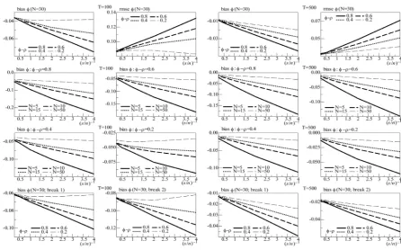
Figure 1. In the figure, Monte Carlo bias and RMSE statistics for the autoregressive parameter (φ) are plotted for the case of

no breaks (top and center plots) and one (break 1) and two (break 2) breaks (bottom plots), and a conditionally heteroskedastic common I(0) factor. Results are reported for various values of the persistence spread φ ‒ ρ (0.2, 0.4, 0.6, 0.8) against various values of the (inverse) signal to noise ratio (s/n)−1 (4, 2, 1, 05, 0.25). The sample size T is 100 and 500 observations, the number of cross-sectional units N is 30, and the number of replications for each case is 2000. For the no breaks case, Monte Carlo bias statistics are also reported for other sample sizes N (5, 10, 15, 50) (center plots).

tional heteroskedasticity, for reasons of space, only the heteroskedastic case is discussed. Moreover, only the results for the φ =d 2 case are reported for the integrated case, as similar results have been obtained for the

0

φ

= case.14

4.1.1. The Structural Stability Case

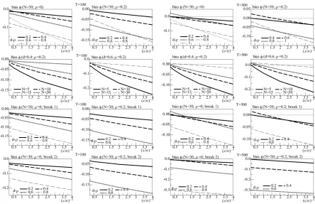
As shown in Figure 5 (top plots 1-4), for a cross-sectional sample size N = 30 units, a negligible downward bias for the

ρ

parameter (on average across (inverse) signal to noise ratio values) can be noted (−0.02 and −0.03, for the non integrated and integrated case, respectively, and T =100 (top plots 1-2); −0.01 and −0.006, respectively, and T =500 (top plots 3-4)), decreasing as the serial correlation spread,

φ ρ

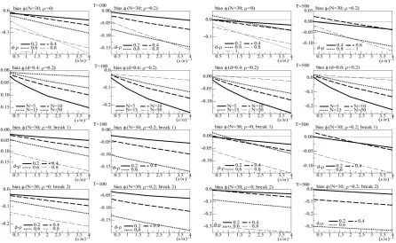
− or d−ρ , or the sample size T increase.

On the contrary, as shown in Figure 1andFigure 3(top plots 1 and 3), the downward bias in φ is increasing with the degree of persistence of the common factor d, the (inverse) signal to noise ratio 𝑠𝑠/𝑛𝑛−1, and the serial correlation spread,

φ ρ

− or d−ρ, yet decreasing with the sample size T.

For the non integrated case (Figure 1, plots 1 and 3), there are only few cases (

φ ρ

− =0.4, 0.6, 0.8) when a 10%, or larger, bias in

φ

is found, occurring when the series are particularly noisy

(

1

)

4

s n− = ; for the stationary long memory case a 10% bias, or smaller, is found for s n−1≥2, while for the non stationary long memory case for s n−1≥1 and a (relatively) large sample (T =500) (Figure 3, plots 1 and 3). Increasing the cross-sectional dimension N yields improvements (see the next section).

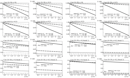
Also, as shown in Figure 2 and Figure 4 (top plots 1-4), very satisfactory is the estimation of the unobserved common stochastic factor, as the IC statistic is always below 0.2 (0.14 (0.10)), on average, for T =100 (T =500) for the non integrated case (Figure 2, top plots 2 and 4); 0.06 (0.03), on average, for T =100 (T =500) for the integrated case (Figure 4, top plots 2 and 4). Moreover, the correlation coefficient between