Computing air demand using the Takagi–Sugeno model for dam outlets

Computing air demand using the Takagi–

Sugeno model for dam outlets

Zounemat­Kermani, M and Scholz, M

http://dx.doi.org/10.3390/w5031441

Title Computing air demand using the Takagi–Sugeno model for dam outlets

Authors Zounemat­Kermani, M and Scholz, M

Type Article

URL This version is available at: http://usir.salford.ac.uk/31837/

Published Date 2013

USIR is a digital collection of the research output of the University of Salford. Where copyright  permits, full text material held in the repository is made freely available online and can be read,  downloaded and copied for non­commercial private study or research purposes. Please check the  manuscript for any further copyright restrictions.

water

ISSN 2073-4441 www.mdpi.com/journal/water Article

Computing Air Demand Using the Takagi–Sugeno Model for

Dam Outlets

Mohammad Zounemat-Kermani 1 _{and Miklas Scholz} 2,_*

1 _{Department of Water Engineering, Shahid Bahonar University of Kerman, Kerman, Iran;} E-Mail: [email protected]

2 _{Civil Engineering Research Group, The University of Salford, School of Computing, Science and} Engineering, Newton Building, Salford, Greater Manchester M5 4WT, UK

* Author to whom correspondence should be addressed; E-Mail: [email protected]; Tel.: +44-161-295-5921; Fax: +44-161-295-5575.

Received: 12 July 2013; in revised form: 13 August 2013 / Accepted: 13 September 2013 / Published: 23 September 2013

Abstract: An adaptive neuro-fuzzy inference system (ANFIS) was developed using the subtractive clustering technique to study the air demand in low-level outlet works. The ANFIS model was employed to calculate vent air discharge in different gate openings for an embankment dam. A hybrid learning algorithm obtained from combining back-propagation and least square estimate was adopted to identify linear and non-linear parameters in the ANFIS model. Empirical relationships based on the experimental information obtained from physical models were applied to 108 experimental data points to obtain more reliable evaluations. The feed-forward Levenberg-Marquardt neural network (LMNN) and multiple linear regression (MLR) models were also built using the same data to compare model performances with each other. The results indicated that the fuzzy rule-based model performed better than the LMNN and MLR models, in terms of the simulation performance criteria established, as the root mean square error, the Nash–Sutcliffe efficiency, the correlation coefficient and the Bias.

Keywords: dam; fuzzy model; outlet works; reservoir; subtractive clustering; Takagi-Sugeno; vent air discharge

Nomenclature

ai = parameter of the consequent part of a rule

A = Area of gate (cm2)

= membership function

ANFIS = adaptive neuro-fuzzy inference system ANN = artificial neural network, also neural network

bi = parameter of the consequent part of a rule

Bias = statistic test representing the mean of all the individual errors

β = aeration coefficient

c = parameter of the consequent part of a rule

Di = density measure

= first cluster center

Fr = Froude number

H = Head of water (cm)

k = index of each fold in the K-fold cross-validation

K = total number of folds in the K-fold cross-validation, and the number of fuzzy ‘if-then’ rules

LMNN = Feed-forward Levenberg-Marquardt artificial neural network Mallows CP = coefficient of the Mallows statistic

MLR = multiple linear regression

= membership degree of the jth input xj for the ith rule

N = number of observations

NSE = Nash–Sutcliffe efficiency (%)

O = opening (%)

Qa = air flow rate (L/s), also called air demand

Oi = measured values of a variable

Qw = Water discharge (L/s)

r = Pearson product moment correlation coefficient, also called correlation coefficient

R0 = positive constant called the cluster radius

ra = influential radius for clustering the data space

rb = positive constant; rb > ra, typically rb = 1.5 ra, where ra is another positive constant

RMSE = root mean square error

Si = computed (by model) values of a variable

Te = true error

TS = Takagi–Sugeno model

ui = normalized degree of fulfilment of the antecedent clause of a rule

Va = air velocity (cm/s)

X = Input vector

= data point with the highest density measure

xn = Input variable

xj = jth input variable in the n dimensional input data space

yi = output variable

i n

A

* 1 D

( )

i

j j

A x

μ

* 1

1. Introduction

1.1. Background

Gated tunnels in dams can be used for various purposes, such as regulating the surface of reservoir water, drawdown of the reservoir, sediment flushing, and flood release [1]. For most dams, flow regulation can be performed from a low level outlet consisting of a closed conduit with a slide gate or valve. Outlet works are devices used to release and regulate water flow from a dam usually for irrigational purposes. Such devices may consist of one or more pipes or tunnels through the embankment of the dam, directing water, often under high pressure, to the river downstream [2]. When the outlet gate is placed inside the conduit, reduced pressure, which may causes cavitation, is often measured just downstream of the gate.

Diffusing air into the flow can eliminate cavitation damages. Aeration will also improve the mean pressure and reduce the intensity of hydrodynamic pressure fluctuations [3]. Therefore, to minimize these effects, aerators are recommended just downstream of gates to introduce air into the flow [4].

A proper size for the air-vent pipe should be considered to allow for the sufficient amount of air flow rate. The air flow rate Qa refers to the amount of air drawn into the air vent. Air flow can be diffused into the water flow through turbulent mixing. The process of air and water mixing can be applied by utilizing a separate air phase above the water surface of the pipe outlet [4].

Insufficient research has been conducted on the air and water flow properties of high-velocity waters discharging at the downstream end of tunnels. Kalinske and Robertson [5] were one of the first researchers who have studied the air demand in closed conduits as a function of the Froude number. Other researchers proposed related but alternative methods for predicting air demand discharge [6–11].

1.2. Purpose, Rationale, Objectives, and Boundary Conditions

The purpose of this study is to apply an adaptive network-based model for air demand estimations regarding low-level outlet works. This work also aims to determine if the use of artificial neural networks (ANN) and simpler models, such as multiple regression models for air demand estimations, could be justified.

In this study, a fuzzy rule-based model was developed for estimating air flow rate in two stages. In the first stage, local sub-regions were determined by analysing the pattern of input data. The regions can be determined intuitively, requiring often too many trial and error attempts. Therefore, alternative clustering techniques were used in this study to find the sub-sets of an input space that characterized possible occurrences of the data. In the second stage, a local model was built for each cluster. The Mamdani’s model, the Takagi–Sugeno’s (TS) model, and the standard additive model can be applied at this stage. In this study, the TS model was chosen, because it can solve complex and high-dimensional problems relying only on a few rules.

process. The dam geometries considered in this research involved a slide gate installed on the sloping upstream face of an embankment dam, followed by a vertical elbow where the flow entered the conduit, as shown in Figure 1. The air demand varied with gate and conduit geometry, gate opening, and water discharge passing through the gate. Hence, these parameters were considered potential input variables for the ANFIS, ANN, and multiple regression models.

Figure 1. Typical representation of a low-level outlet works.

2. Materials and Methods

2.1. Experimental Data

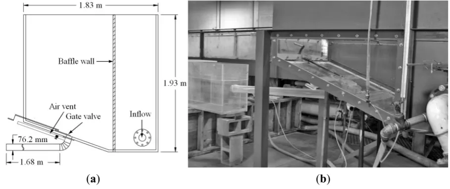
The 108 data used in this study were obtained from a study published by Tullis and Larchar [4]. In an effort to develop a better understanding of head-discharge relationships and air-venting requirements for inclined slide gates, a laboratory-scale model (Figure 2) of low-level outlet works representative of small- to medium-sized embankment dam applications was constructed at the Utah Water Research Laboratory, Utah State University. A schematic representation of the experimental set-up is shown in Figure 2b. The model shown in Figure 2a consisted of an elevated steel tank (approximately 1.8 m long, 1.8 m tall and 0.9 m wide). Two acrylic slide gates (round and rectangular) were constructed and subsequently tested. The gate designs were based on commercially available slide gates. The data collected for each test condition included the area of gate (A), opening percentage (O%), head of water (H), and water discharge (Qw) for outlet conditions and the air velocity (Va) in the supply line (vented only).

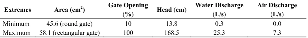
Table 1. Design parameters after [4].

Extremes Area (cm2) Gate Opening

(%) Head (cm)

Water Discharge

(L/s)

Air Discharge

(L/s)

Minimum 45.6 (round gate) 10 13.8 0.3 0.0

Maximum 58.1 (rectangular gate) 100 168.5 25.3 7.3

Figure 2. (a) Schematic of lab-scale low-level outlet works; and (b) experimental set-up after [4].

(a) (b)

2.2. Empirical Relationships for Estimating Discharge Air Vents

Research has traditionally concentrated on the flow aeration downstream of bottom outlet gates. Studies are usually based on experimental information obtained from physical models. Most of the published air-venting studies are limited to large-dam outlet geometries [4]. In order to validate the experimental relationships for low-level outlets, formulas related to large dam outlets were considered for determining the air demand in this study.

The Froude Number is a dimensionless parameter defined as the ratio of a characteristic velocity to a gravitational wave velocity [Equation (1)]. Kalinske and Robertson [5] reported results on air demand for situations where a hydraulic jump was formed in the downstream conduit. Based on their results, the aeration coefficient (β) for the condition of a hydraulic jump was suggested as a function of the Froude number (Fr) as shown in Equation (2).

(1)

where Fr is the Froude number; V is the mean velocity of water; Yc is the flow depth at the contracted section; and g is the gravitational acceleration.

(2)

The aeration coefficient (β) can also be expressed as the vent air discharge over the water flow discharge (β = Qa/Qw). Campbell and Guyton [6] presented Equation (3) for the air demand ratio using the Froude number in the contracted section downstream of the gate [12].

(3)

The U.S. Army Corps of Engineers [7] published Equation (4), which is based on prototype observations. Equation (4) is rather similar to Equation (3).

(4) .

= c V Fr

g Y

(

)

0.0066 1

β

(

)

0.04 1

β = Fr−

(

)

0.03 1

In another experiment, Sharma [10] verified prototype data and compared results with the empirical equations in the water flow of conduits. Equation (5) directly relates the aeration coefficient to the Froude number according to Sharma’s experiments.

(5)

2.3. Adaptive Network-Based Fuzzy Inference System

The ANFIS integrates the features of fuzzy systems and neural networks. Thereafter, it has the potential to capture the benefits of both in a single framework. Membership functions are the central concept of fuzzy set theory, which numerically represents the degree to which a given element belongs to a fuzzy set [13].

In order to avoid over-fitting of the ANFIS model, an early stopping technique has been applied. In this method, the validation set can be used to detect the time in which over-fitting starts during the supervised training. At this stage, training is stopped before convergence to avoid over-fitting [14].

2.4. Takagi–Sugeno’s Model

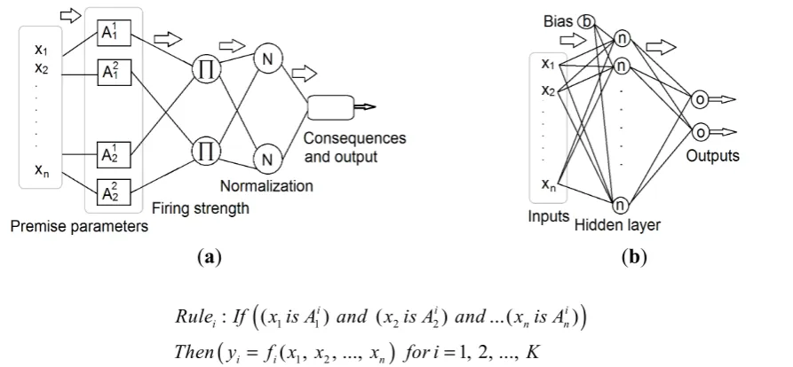
The TS model was published by Takagi and Sugeno in 1985 [15]. A TS fuzzy model consists of four major elements of member functions, internal functions, rules, and outputs [16]. The TS fuzzy models are quasi-linear in nature, resulting in smooth transitions between linear sub-models [17]. Figure 3a illustrates the typical structure of the ANFIS model. For a multi-input and single-output model, the typical fuzzy rule of a TS model is shown in Equation (6).

Figure 3. Schematic representation of the (a) adaptive neural-based fuzzy inference system; and the (b) feed-forward Levenberg-Marquardt artificial neural network structure.

(a) (b)

(6)

where xn is the input variable, is the membership function (MF) and K is the number of fuzzy if-then rules. The consequent part of the rule base shows the rule output. In a TS fuzzy model, rule consequents are usually taken to be either crisp numbers or linear functions of the input parameters [Equation (7); layer 1].

0.09

β = Fr

(

)

(

)

1 1 2 2

1 2

: ( ) ( ) ...( )

( , , ..., 1, 2, ...,

i i i

i n n

i i n

Rule If x is A and x is A and x is A

(7)

where yi is the output variable, and ai and c are parameters of the consequent parts of the rule shown in Equation (6). The number of rules is indicated by K, and Ai is the antecedent fuzzy set of the i-th rule defined by the membership function (premise parameters in Figure 3a). The degree of matching between the input parameters and rule [Equation (6)] is called the rule firing strength (Figure 3a), which is normally defined as an and-conjunction by means of the product operator [Equation (8); layer 2].

(8)

where xj is the j-th input variable in the n dimensional input data space and is the membership

degree of the j-th input xj for the i-th rule. For the input x, the total output y of the TS model is computed by aggregating the contributions of individual rules [17]. Therefore, the overall fuzzy system output can be obtained by Equation (9). Consequents and outputs are shown in Figure 3a.

(9)

where ui is the normalized degree of fulfilment of the antecedent clause of rule shown in Equation (6) [13,18]. The normalized degree of fulfilment can be expressed by Equation (10). The normalization layer is shown in Figure 3a.

(10)

2.5. Hybrid Algorithm

Two learning methods are generally used in the adaptive TS model to specify the relationship between input and output and to determine the optimized distribution of MF. The TS model utilizes a combination of the least-square method and the back-propagation gradient descent method for training the FIS membership function parameters to identify patterns hidden in a given training dataset [19–22]. Several methods can be utilized for setting up the MF of the ANFIS (e.g., grid partition and subtractive clustering). Regarding the combination of grid partition and ANFIS, grid partition divides the input vector into a number of fuzzy regions using paralleled axis. However, in this method, fuzzy rules increase exponentially when the amount of input variables increases. Therefore, the application of grid partition in ANFIS is not recommended for large input variable problems [23].

In this study, a subtractive clustering method was used to initialize the Gaussian type of MF. The simulation begins by generating the fuzzy rules using subtractive clustering, which is based on a measure of the density of data points in the feature space. This approach is applied to determine the number of rules and antecedent membership functions by considering each cluster centre as a fuzzy rule. An example of how the clusters are identified in the second (gate opening) and the fourth (water discharge) input dimensions as well as the third (head of water) and fourth (water discharge) input dimensions of the input space is shown in Figure 4.

1 2 1 1 2 2

1 1 2 2

( , ,..., ) ... ...

i i i i

i i n n n

i i i i

i n n

y f x x x a x a x a x c y a x a x a x c

= = + + + + = + + + + i j A μ 1 ( ) i j n

i A j

j x α μ = =∏ ( ) i j j A x μ 1 ( ). K i i i

y u x y

Figure 4. Cluster centres using the centre of gravity method in (a) input 2 [gate opening (O)] and input 4 [water discharge (Qw)]; and in (b) input 3 [head of water (H)] and input 4 (Qw).

Desirable variables of the membership functions are optimized for the identification data set through the back-propagation procedure while a linear least squares method is used for calculating the consequent parameters. Parameters associated with membership functions change through the learning process and the gradient vector facilitates the calculation of these parameters. Each time when the gradient vector is obtained, an optimization procedure is performed to adjust parameters for reducing errors [24].

2.6. Input Data Determination

The selection of appropriate input variables is an important consideration in heuristic modeling. Inappropriate input variable selection may cause unsuitable effects on the modelling results. Several remedies were reported to overcome these problems including autocorrelation and partial autocorrelation function analysis, linear and non-linear cross-correlation analysis, spectral analysis, and partial mutual information [25,26].

In the study, input variables are selected using a stepwise selection procedure. A stepwise regression method (i.e., step-by-step iterative construction of a regression model that involves automatic selection of independent variables) was applied to explore relationships among the collected data. The Mallows statistic was used as a criterion to select a suitable multiple regression model. Mallows CP is a powerful selection procedure in stepwise regression [27]. The result of stepwise regression according to Mallows CP coefficient is tabulated in Table 2.

According to findings shown in Table 2, the area representing the shape of the slide gate (round or rectangular) was found to be the most significant variable for explaining air discharge demand.

Table 2. Stepwise regression results for the four independent variables area of gate (A), head of water (H), opening percentage (O) and water discharge (Qw) against the dependent parameter of air flow rate (Qa).

Step 1 2 3 4

Parameter A (cm2_{) H (cm) Qw (L/s) O (%)}

However, water head and water discharge followed by gate opening percentage were also found to be significant as input variables. Therefore, both artificial intelligence models (fuzzy and ANN) as well as the regression model were tested using all available explanatory variables.

2.7. Comparing Model Performance

The performance of the developed models can be evaluated using several statistical tests that describe the errors associated with the model. After calibrating each model structure using the testing data set, the performance can then be evaluated in terms of statistical measures of goodness of fit. In order to provide an indication of goodness of fit between the observed and estimated values, the root mean square error (RMSE), correlation coefficient (r), Nash–Sutcliffe efficiency (NSE), and Bias were calculated and evaluated. The RMSE evaluates the variance of errors independently from the sample size, which is given by Equation (11).

(11)

where Si and Oi represent the model computed and measured values of the variable; and N indicates the number of observations. The smaller the RMSE, the better is the performance of the model. The Bias represents the mean of all the individual errors and indicates whether the model overestimates or underestimates the dependent variable. This statistic is calculated as shown in Equation (12) [28,29].

(12)

The NSE, which is a normalized statistic, determines the relative magnitude of residual variance compared to the observed variance and gives an indication of how well the observed and simulated results fit to a 1:1 line (line of agreement). This statistic can be obtained via Equation (13) [30].

(13)

NSE ranges from −∞ to 1. Essentially, the closer NSE is to 1, the more accurate the model is likely to be. The correlation coefficient (r) is based on the Pearson product moment correlation coefficient of the simulated and observed flow series, which is obtained via Equation (14).

(14)

The correlation coefficient is a measure of strength of the model in developing a relationship between input and output variables. The higher the r value (with 1 being the maximum value), the better is the performance of the model.

2.8. K-fold Cross-Validation

Cross validation techniques tend to focus on not using the entire data set when building a model. They are applied for assessing how the results of statistical analysis would generalize to an

2

1

1 N _{( )} i i i

RMSE _N S O

= =



(

)

Bias S O

N =

=



(

)

(

)

1 1

1 n i i / n i i

i i

NSE S O O O

= =   = −_ − − _ 





(

)(

)

(

)

(

)

i i i i

i

n n

o s

i i i

i i

O O S S r

independent data set. In addition, they are applied for the settings in which the goal is estimating how accurately a predictive model would perform in practice. In K-fold cross-validation, the data are split into K parts (folds) with K-1 parts as the training set and one part as the testing set.

The cross-validation process is then repeated K times. Once the model is built using the left cases (often called the training data set), the cases that are removed (referred to as the testing data set) can be used to test the performance of the model on the ‘unseen’ data (i.e., the testing set). The K results from the folds can then be averaged (or otherwise combined) to produce a single estimation [31].

The advantage of this strategy is that all data have the chance to be trained and evaluated, giving the true error (Te) for each error criterion (RMSE, Bias, NSE, and r). Equation (15) shows the true error of the RMSE:

(15)

where K is the total number of folds and k is the index of each fold. In this study, the data set was divided randomly into four training and testing sub-sets by the cross validation method as a systematic process to obtain effective and sensitive modelling results.

3. Results and Discussion

3.1. Applications

It is expected that training data sets should cover all the characteristics of the scientific problem to obtain correct model estimations. Therefore, the data set was divided into four training and testing sub-sets by using the cross validation method as a systematic methodology to obtain effective and sensitive model findings. To get more reliable evaluations of performance of the ANFIS model, MLR given in Equation (16) was established for the 108 experimental data [32]. As with the fuzzy approach, the four-fold cross validation method was used again.

(16)

The best model structure having four input variables was also trained and tested by ANN. The feed-forward Levenberg-Marquardt ANN network (LMNN) was used in this study. The LMNN model was trained and tested using the same non-transformed data set. The error back-propagation algorithm and tangent activation function were used for the training/testing of the LMNN model. Figure 3b shows the typical schematic representation of a LM back-propagation neural network. The number of hidden layers and the hidden neurons within a layer, the learning rate (0.1), the coefficient of momentum (0.5) and epochs (1000) were selected by applying a trial and error method during the model training phase. The structure of the LMNN model consisted of eleven hidden neurons within one hidden layer. Details on the development of the LMNN model were presented in previous reports [14,33]. Table 3 summarizes the comparison of results of the ANFIS, LMNN, MLR, and empirical models.

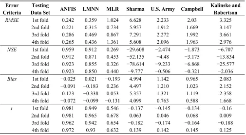
Comparing the estimation models from Table 3, it can be seen that RMSE values with respect to the ANFIS model were much lower compared to the MLR and empirical models for each fold. The RMSE values of the ANFIS model were also lower than those for the LMNN model. In addition, values for the NSE efficiency and correlation coefficients of the ANFIS model were higher than those for the

1

1 K

Te k

k

RMSE _K RMSE

=

 

= _{ }





[

]

a w

LMNN, MLR and empirical models for each fold. However, it should be noted that a trial and error procedure had to be performed for the LMNN model to develop the best network structure while such a procedure was not required for developing the ANFIS model. Moreover, in this study, the ANFIS model was trained using just 30 epochs while the LMNN model required 60 epochs. The results suggest that the ANFIS method was superior to the LMNN method in estimating the vent air discharge.

Table 3. Values of model performance indices and error functions for the testing.

Error Criteria

Testing

Data Set ANFIS LMNN MLR Sharma U.S. Army Campbell

Kalinske and Robertson

RMSE 1st fold 0.242 0.359 1.024 6.628 2.233 2.03 3.325

2nd fold 0.221 0.315 0.734 5.957 1.912 1.669 3.147

3rd fold 0.286 0.469 0.867 7.291 2.272 1.992 3.661

4th fold 0.265 0.436 1.361 5.608 2.096 1.963 2.976

NSE 1st fold 0.959 0.912 0.269 −29.608 −2.474 −1.873 −6.707 2nd fold 0.912 0.871 0.453 −52.135 −4.48 −3.175 −13.834 3rd fold 0.923 0.855 0.326 −78.614 −9.233 −6.868 −25.577 4th fold 0.923 0.850 0.440 −9.777 −0.506 −0.321 −2.036

Bias 1st fold −0.025 0.021 −0.193 4.994 1.142 0.965 2.083

2nd fold −0.091 −0.183 0.236 4.497 1.210 1.023 2.152

3rd fold 0.123 −0.338 0.053 5.357 1.321 1.119 2.358

4th fold −0.072 −0.099 −0.131 4.099 0.763 0.588 1.668

r 1st fold 0.981 0.949 0.546 −0.137 −0.145 −0.134 −0.16

2nd fold 0.981 0.965 0.678 0.063 0.046 0.068 0.009

3rd fold 0.962 0.942 0.654 −0.182 −0.174 −0.164 −0.188

4th fold 0.972 0.93 0.632 0.139 0.142 0.145 0.125

Notes: ANFIS, adaptive neural-based fuzzy inference system; LMNN, feed-forward Levenberg-Marquardt

artificial neural network; MLR, multiple linear regression; RMSE, root mean square error; NSE, Nash–Sutcliffe

efficiency; Bias, test statistic representing the mean of all the individual errors; r, Pearson product moment

correlation coefficient.

Scatter plots are displayed in Figures 5 and 6 for the training and testing data sets, respectively. Figure 6 shows the observed vent air discharge on the x-axis against the simulated vent air discharge on the y-axis for the Campbell and Kalinske-Robertson’s empirical relationships.

Figure 5. Comparing the results of Campbell and Kalinske-Robertson’s empirical models versus the observations (1st fold).

Figure 6. Comparing the results of adaptive neural-based fuzzy inference system (ANFIS) and multiple linear regression (MLR) models versus the observations (testing set of 1st fold).

3.2. Assessing Empirical, ANFIS, MLR, and LMNN Models

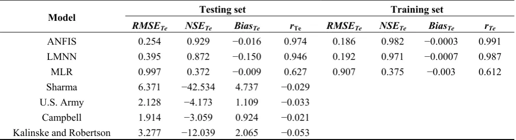
For comparison, performance data of the ANFIS model against the corresponding MLR and empirical models are presented in Table 4 using true error values. It is evident that the ANFIS model was by far more accurate than the empirical models and considerably more accurate than the MLR and LMNN models in terms of their simulation accuracy of the true error criteria. The ANFIS model simulated the significant air discharge parameters with an acceptable accuracy. The result of the Bias index indicated that all empirical relationships highly overestimated air discharges (e.g., BiasTE for Sharma = 4.7) while the LMNN model slightly underestimated air discharges (BiasTE = −0.15). ANFIS and MLR had normal tendencies with negligible magnitude for Bias. The overall average values for NSE were slightly negative.

Table 4. Performance statistics for the adaptive neural-based fuzzy inference system (ANFIS), feed-forward Levenberg-Marquardt artificial neural network (LMNN), multiple linear regression (MLR), and empirical models using true error (Te).

Model Testing set Training set

RMSETe NSETe BiasTe rTe RMSETe NSETe BiasTe rTe

ANFIS 0.254 0.929 −0.016 0.974 0.186 0.982 −0.0003 0.991

LMNN 0.395 0.872 −0.150 0.946 0.192 0.971 −0.0007 0.987

MLR 0.997 0.372 −0.009 0.627 0.907 0.375 −0.003 0.612

Sharma 6.371 −42.534 4.737 −0.029

U.S. Army 2.128 −4.173 1.109 −0.033

Campbell 1.914 −3.059 0.924 −0.021

Kalinske and Robertson 3.277 −12.039 2.065 −0.053

Notes: RMSE, root mean square error; NSE, Nash–Sutcliffe efficiency; Bias, test statistic representing the

mean of all the individual errors; r, Pearson product moment correlation coefficient.

For the ANFIS model, NSETe is 0.93, which corresponds to a perfectly modeled match to the observed data, indicating the superiority of the ANFIS model compared to both the LMNN and MLR approaches. Negative values of NSE indicated that the observed mean was a better predictor than the model. Thereafter, all the empirical models failed to simulate the air discharges properly according to the NSE criteria. In general, the results suggested that the ANFIS method is superior to the LMNN, MLR, and empirical methods for the purpose of simulating vent air discharges.

3.3. Comparison between Empirical and Computational Methods

According to empirical relationships, the air demand flow at different gate opening scenarios was determined as function of the Froude number at a contracted section according to Equations (2–5). Findings have subsequently been compared with computational relations.

Results indicate that there are considerable differences between empirical and computational methods. This could be explained by differences in the input variables used by each method. The Froude number [Equation (1)], which is used by all empirical methods as the basic parameter for estimating the air demand, includes velocity (V) as a dependent parameter of water discharge, gate opening, and vent area ( = / ∙ ) and the flow depth at the contracted section, which is a dependent parameter of water depth and gate opening ( = ∙ ). Therefore, the empirical relationships are a function of four parameters: ( , , , ). According to the stepwise regression results (Table 2), the second most effective input variable of estimating air flow rate is head of water (H), which is not an input variable for the empirical relationships. This could be the reason for inferior results associated with the empirical relationships in comparison to the computational methods.

In addition to the empirical relationships, experimental data were used to assess the relationship based on non-linear regression between the Froude number (Fr) and the aeration coefficient (β). Equation (17) shows the best power relationship for the applied experimental data (Figure 7).

(17)

1.85

0.08(Fr 1)

Figure 7. Illustration of the power relationship between the Froude number (Fr) and the aeration coefficient (β) of the applied experimental data.

In order to evaluate the validity of the above relationships, the statistical measures RMSE, NSE, Bias and r were calculated. Results show that the RMSE = 1.24, NSE = −0.14, Bias = −0.00036 and r = −0.045. Comparing the performance of the obtained relationships to the empirical ones [Equations (2–5)] indicates their superiority (lower RMSE, r and normal tendency for Bias) to other empirical power relationships discussed in this study. However, it should be noted that artificial intelligence models (e.g., ANFIS and ANN) do not provide an explicit expression relating the independent with the dependent variables.

4. Conclusions

Fuzzy modelling and identification of measured data are effective tools for the approximation of uncertain non-linear systems. In this paper, a TS fuzzy inference system was successfully developed and applied for the simulation of air demand discharge in low-level dam outlet works. The subtractive clustering algorithm was utilized to extract the fuzzy model structure. In order to verify the performance of the proposed approach, empirical methods (Shrama, Campbell, Kalinske-Robertson, and U.S. Army), a traditional MLR model and the more recent LMNN model were successfully built using the same data and subsequently compared with each other. The data were randomly separated into four sub-sets using the K-fold cross validation method.

The performances of the empirical models were inferior to the MLR model. The Bias index values indicated that empirical methods highly over-estimated the air demand discharges while the ANFIS model had a normal tendency. The average RMSE of four folds was 0.25 for the ANFIS model compared to 0.40 for the LMNN model, which was considered acceptable. The performance of the ANFIS model was satisfactory, considering that the average NSE efficiency values of 0.98 and 0.93 were recorded for the training and testing data sets, respectively. Lower corresponding values of NSE efficiency were computed for the LMNN (0.97/0.87) and MLR (0.38/0.37) models.

MLR, and artificial neural network models to assess the interactions between air demand discharge and hydro-structural parameters of low-level outlet works for dams.

Conflicts of Interest

The authors declare no conflict of interest.

References

1. Vischer, D.L.; Hager, W.H. Dam Hydraulics; John Wiley & Sons: Chichester, UK, 1998.

2. Larchar, J.A. Air Demand in Low-level Outlet Works. MSc Thesis, Utah State University, Logan, UT, USA, 12 January 2011.

3. Kavianpour, M.R.; Rajabi, E. Application of neural network for flow aeration downstream of outlet leaf gates. Iran Water Resour. Res. 2005, 1, 1–8.

4. Tullis, B.P.; Larchar, J. Determining air demand for small- to medium-sized embankment dam low-level outlet works. J. Irrig. Drain. Eng. 2011, 137, 793–800.

5. Kalinske, A.A.; Robertson, J.W. Closed conduit flow. ASCE Trans. 1943, 108, 1435–1447.

6. Campbell, F.B.; Guyton, B. Air demand in gated outlet works. In Proceedings of the 5th International Association for Hydraulic Research (IAHR) and American Society of Civil Engineers (ASCE) Joint, Reston, VA, USA, 1–4 September 1953; pp. 529–533.

7. U.S. Army Corps of Engineers (USACE). Hydraulic Design Criteria: Air Demand-regulated Outlet Works; USACE: Washington, DC, USA, 1964.

8. Wisner, P. On the role of the froude criterion for the study of air entrainment in high velocity flows. In Proceedings of the 11th International Association for Hydraulic Research (IAHR Congress), Madrid, Spain, 6–11 September 1965.

9. U.S. Bureau of Reclamation (USBR). Hydraulic Model Studies of the Silver Jack Outlet Works Bypass; Bostwick Park Project; USBR: Denver, CO, USA, 1966.

10. Sharma, H.R. Air-entrainment in high head gated conduits. J. Hydraul. Div. 1976, 102, 1629–1646.

11. Ozkan, F.; Baylar, A.; Ozturk, M. Air entrainment and oxygen transfer in high-head gated conduits. Proc. Inst. Civ. Eng. Water Manag. 2006, 159, 139–143.

12. Yazdi, J.; Zarrati, A.R. An algorithm for calculating air demand in gated tunnels using a 3D numerical model. J. Hydro Environ. Res. 2011, 5, 3–13.

13. Vernieuwe, H.; Georgieva, O.; de Baets, B.; Pauwels, V.R.N.; Verhoest, N.E.C.; de Troch, F.P. Comparison of data-driven Takagi-Sugeno models of rainfall-discharge dynamics. J. Hydrol. 2005, 302, 173–186.

14. Zounemat-Kermani, M. Hourly predictive Levenberg-Marquardt ANN and multi linear regression models for predicting of dew point temperature. Meteorol. Atmos. Phys. 2012, 117, 181–192. 15. Takagi, T.; Sugeno, M. Fuzzy identification of systems and its applications to modeling and

control. IEEE Trans. Syst. Man Cybern. 1985, 15, 116–132.

17. Lohani, A.K.; Goel, N.K.; Bhatia, K.K.S. Takagi-Sugeno fuzzy inference system for modeling stage-discharge relationship. J. Hydrol. 2006, 331, 146–160.

18. Torun, Y.; Tohumoglu, G. Designing simulated annealing and subtractive clustering based fuzzy classifier. Appl. Soft Comput. 2011, 11, 2193–2201.

19. Talebizadeh, M.; Moridnejad, A. Uncertainty analysis for the forecast of lake level fluctuations using ensembles of ANN and ANFIS models. Exp. Syst. Appl. 2011, 38, 4126–4135.

20. Pulido-Calvo, I.; Gutiérrez-Estrada, J.C. Improved irrigation water demand forecasting using a soft-computing hybrid model. Biosyst. Eng. 2009, 102, 202–218.

21. Zhang, G.P. Time series forecasting using a hybrid ARIMA and neural network model. Neurocomputing 2003, 50, 159–175.

22. Zounemat-Kermani, M.; Teshnehlab, M. Using adaptive neuro-fuzzy inference system for hydrological time series prediction. Appl. Soft Comput. 2008, 8, 928–936.

23. Cobaner, M. Evapotranspiration estimation by two different neuro-fuzzy inference systems. J. Hydrol. 2011, 398, 299–302.

24. Wu, X.J.; Zhu, X.J.; Cao, G.Y.; Tu, H.Y. Nonlinear modeling of a SOFC stack based on ANFIS identification. Simul. Model. Pract. Theory 2008, 16, 399–409.

25. Pulido-Calvo, I.; Gutiérrez-Estrada, J.C.; Savic, D. Heuristic modelling of the water resources management in the Guadalquivir River Basin, Southern Spain. Water Resour. Manag. 2012, 26, 185–209.

26. Fernando, T.M.K.G.; Maier, H.R.; Dandy, G.C. Selection of input variables for data driven models: An average shifted histogram partial mutual information estimator approach. J. Hydrol. 2009, 367, 165–176.

27. Kadane, J.B.; Lazar, N.A. Methods and criteria for model selection. Am. Statist. Assoc. 2004, 99, 279–290.

28. Singh, K.P.; Basant, A.; Malik, A.; Jain, G. Artificial neural network modeling of the river water quality—A case study. Ecol. Modell. 2009, 220, 888–895.

29. Adamowski, J.; Karapataki, C. Comparison of multivariate regression and artificial neural networks for peak urban water-demand forecasting: Evaluation of different ANN learning algorithms. J. Hydrol. Eng. 2010, 15, 729–743.

30. Katambara, Z.; Ndiritu, J.G. A hybrid conceptual-fuzzy inference streamflow modelling for the Letaba River system in South Africa. Phys. Chem. Earth 2010, 35, 582–595.

31. Firat, M.; Güngör, M. River flow estimation using adaptive neuro fuzzy inference system. Mathem. Comput. Simul. 2007, 75, 87–96.

32. Dursun, O.F.; Kaya, N.; Firat, M. Estimating discharge coefficient of semi-elliptical side weir using ANFIS. J. Hydrol. 2012, 426–427, 55–62.

33. Zounemat-Kermani, M. Hydrometeorological parameters in prediction of soil temperature by means of artificial neural network: Case study in Wyoming. J. Hydrol. Eng. 2013, 18, 707–718.