BIROn - Birkbeck Institutional Research Online
Pesaran, M.H. and Smith, Ron P. (2014) Counterfactual analysis in
macroeconometrics: an empirical investigation into the effects of quantitative
easing. Working Paper. Birkbeck College, University of London, London, UK.
Downloaded from:
Usage Guidelines:
Please refer to usage guidelines at or alternatively
Counterfactual Analysis in Macroeconometrics: An Empirical
Investigation into the E¤ects of Quantitative Easing
M. Hashem Pesaran
University of Southern California and Trinity College Cambridge Ron P Smith
Birkbeck, University of London
June 2014
Abstract
The policy innovations that followed the recent Great Recession, such as unconventional monetary policies, prompted renewed interest in the question of how to measure the e¤ective-ness of such policy interventions. To test policy e¤ectivee¤ective-ness requires a model to construct a counterfactual for the outcome variable in the absence of the policy intervention and a way to determine whether the di¤erences between the realised outcome and the model-based counter-factual outcomes are larger than what could have occurred by chance in the absence of policy intervention. Pesaran & Smith (2014b) propose tests of policy ine¤ectiveness in the context of macroeconometric rational expectations dynamic stochastic general equilibrium models. When we are certain of the speci…cation, estimation of the complete system imposing all the cross-equation restrictions implied by the full structural model is more e¢ cient. But if the full model is misspeci…ed, one may obtain more reliable estimates of the counterfactul outcomes from a parsimonious reduced form policy response equation, which conditions on lagged values, and on the policy measures and variables known to be invariant to the policy intervention. We propose policy ine¤ectiveness tests based on such reduced forms and illustrate the tests with an application to the unconventional monetary policy known as quantitative easing (QE) adopted in the UK.
Keywords: Counterfactuals, policy analysis, policy ine¤ectiveness test, macroeconomics, quantitative easing (QE)
JEL classi…cation: C18, C54, E65,
1
Introduction
The Great Recession that followed the …nancial crisis starting in 2007 prompted a range of
pol-icy innovations. These included unconventional monetary policies and increased …scal activism,
through either stimulus or austerity measures depending on the country concerned. These
inno-vations have prompted renewed interest in the question of how one measures the e¤ectiveness of
such policy interventions. To test policy e¤ectiveness requires a model to construct a
counterfac-tual for the outcome variable in the absence of the policy intervention and a way to determine
whether the di¤erence between the realised outcome and the counterfactual outcome is larger
than one would expect by chance. In a companion paper, Pesaran & Smith (2014b), PS, we
pro-pose asymptotic tests for the null hypothesis of policy ine¤ectiveness in the context of complete
systems of macroeconometric dynamic stochastic general equilibrium (DSGE), rational
expecta-tions, RE, models. In this paper we consider testing for the e¤ectiveness of policy using "reduced
form policy response equations" rather than full structural models. We pay particular attention
to the speci…cation of the counterfactual and the role of endogenous and exogenous conditioning
variables. As an illustration, we test for the e¤ectiveness of the unconventional monetary policy
known as quantitative easing (QE) adopted in March 2009 in the UK.
When we are reasonably con…dent in the speci…cation, estimation of the complete system
imposing all the cross-equation restrictions implied by the structural DSGE model yields more
reliable estimates of the counterfactual outcomes as compared to using the reduced form
speci…-cations. However, we are rarely certain of the correct speci…cation for the complete system and if
the full model is misspeci…ed, more robust estimates of the counterfactuals may be obtained from
a reduced form policy response equation for the variable of interest. Since a counterfactual is a
type of forecast, and parsimonious models tend to forecast better, using a small policy model to
construct the counterfactual outcomes might even be preferable to using a large structural models,
where one may be more liable to misspeci…cation of some equations with adverse consequences for
the quality of counterfactual outcomes reliability of the other equations. Accordingly, we propose
tests for policy ine¤ectiveness based on such reduced forms.
As in PS, we consider a policy intervention which takes the form of a change in one or
more of the parameters of a policy rule. The tests are then based on the di¤erences, over a
given policy evaluation horizon, between the post-intervention realizations of the policy target(s)
and associated counterfactual outcomes based on the parameters estimated using data before
the policy intervention. The Lucas Critique is not an issue since the counterfactual, given by
the predictions from the model estimated on pre-intervention data, will embody pre-intervention
policy, the change in parameters and the consequent change in expectations. The development of
the test does not require knowing the post-intervention parameters.
We are concerned with ex post evaluation of a policy intervention on a single unit (country), where data are available before and after the intervention. Di¤erent issues are involved inex ante
policy formulation where post-intervention data are not available and the Lucas Critique could
be an issue since the possible e¤ects of the policy change on parameters and expectations must be
taken into account. We develop tests of policy ine¤ectiveness and derive their asymptotic
distri-butions both when the post-intervention sample is …xed as the pre-intervention sample expands,
and when both samples rise jointly but at di¤erent rates and investigate the power of the tests.
In the case of static reduced forms we also derive an exact test.
The concept of counterfactual used in the development of our proposed test refers to
hypothet-ical outcomes obtained under the null of policy ine¤ectiveness and is, therefore, more narrowly
de…ned than in the literature. The term "counterfactual" has a variety of distinct, though
con-nected, uses in philosophy, history, economics and statistics. In philosophy counterfactual
scenar-ios are often used in the analysis of causality, e.g. Lewis (1973). Pearl (2009) provides an overview
of the concepts and develops an analysis of causality based on structural models. In history
coun-terfactuals are posed by "what if" questions, such as "what would the U.S. economy have been
like in 1890 had there been no railroads?", Fogel (1964). In economics alternative counterfactuals
(hypothetical states of the world) are considered in decision making under uncertainty. In
statis-tics and econometrics counterfactuals are used in medical trials and microeconometric program
evaluations. These uses, whilst connected, are quite distinct and the appropriate de…nition of a
counterfactual crucially depends on the context.
Counterfactuals have been used to examine a range of macroeconometric questions. Abadie
and Gardeazabal (2003) examine the e¤ect of terrorism on the Basque country using a "synthetic
control region" to provide a counterfactual. Pesaran, Smith and Smith (2007) examine what would
have happened to the economies of the UK and the eurozone had the UK joined the euro in 1999,
using "euro" restrictions on a GVAR model to construct counterfactual outcomes. Hsiao, Ching
and Wan (2011) examine the e¤ect on output growth in Hong Kong of political and economic
integration with mainland China, constructing counterfactuals based on predictions from similar
economies. Fagan, Lothian and McNelis (2013) examine whether the Gold Standard was really
destablising, constructing the counterfactual by replacing the pre-1914 US money supply process
with a Taylor rule in a DSGE model.
Whereas there is a large literature on microeconometric policy evaluation that focuses on the
measurement and testing of treatment e¤ects, surveyed, for example, by Imbens and Wooldridge
eval-uation. The micro and macro issues are rather di¤erent. For instance, the endogeneity and sample
selection bias that arise due to correlated heterogeneity across the units in the micro-treatment
case is not a problem in the macro case when the focus of the policy evaluation is on a single
unit, and the "policy on/policy o¤" comparisons are done over time rather than across units. In
micro terminology, the parameter of interest in the macro cases is the e¤ect of treatment on the
treated: it makes no sense to consider either the e¤ect of Hong Kong joining the euro or of the
UK being integrated with China.
Another recent approach to macro policy evaluation borrows techniques from the micro
liter-ature to obtain an estimate of an average treatment e¤ect. Angrist, Jorda and Kuersteiner (2013,
AJK), drawing on Angrist and Kuersteiner (2011), estimate the e¤ect of monetary policy, while
Jorda and Taylor (2013) use similar procedures to estimate the e¤ect of …scal policy. AJK use
local linear projection type estimators to measure the average e¤ect of policy changes on future
values of the outcome variables (in‡ation, industrial production, and unemployment), weighted
inversely by policy propensity scores in a way similar to that used to adjust non-random samples.
Their approach di¤ers from the one proposed in this paper in two important respects. First,
they rely on outcomes averaged across di¤erent (possibly heterogenous) policy episodes whilst we
consider a single policy intervention and average the counterfactual outcomes for the same post
intervention sample. Second, AJK do not use a structural model and their analysis is subject
to the Lucas Critique. Their approach requires that the underlying parameters are invariant to
policy changes, since it is only policy changes within the same regime that are identi…ed in their
framework (see AJK, p.5). In addition, matching estimators of this sort require a lot of data
whereas macroeconometric samples tend to be data-poor relative to microeconometric samples.
This is re‡ected in the large con…dence bands AJK report around the measures of their estimated
e¤ects of target rate changes on macro variables.
We use the policy ine¤ectiveness tests to investigate the e¤ects of the QE introduced in the
UK after March 2009 To this end we employ an autoregressive distributed lag (ARDL) equation
in the target variable, output growth (yt) , the policy variable, the spread between long and
short rates (xt), and US and euro area output variables, wt; that we assume to be invariant to
the policy change. We exclude endogenous variables, zt; that could in‡uence yt both directly
or through the changes in xt: For instance, it would be wrong to include the exchange rate in
the equation, because if QE was e¤ective in reducing the spread then the exchange rate would
almost certainly have been changed by it and we would have needed to allow for that e¤ect by
considering a separate equation that links the exchange rate toxt. By excluding the exchange rate
from the policy response equation we are in e¤ect replacing the exchange rate by its determinants
change. This is the reverse of the usual misspeci…cation argument, since we wish to attribute to
xt the e¤ects that are transmitted throughzt:It is not a question ofceteris paribus, other things
being equal, held constant, butmutatis mutandis, changing what needs to be changed.1 We …nd that a 100 basis points reduction in the spread (due to the QE) has an impact e¤ect on output
growth of about one percentage point, but the policy impact is very quickly reversed.
The rest of the paper is organized as follows: Section 2 sets up a DSGE model with
exoge-nous variables and derives its solution which is the basis for the reduced form policy response
equations we estimate. Section 3 develops the policy ine¤ectiveness tests. Section 4 considers the
empirical application to investigate the e¤ectiveness of the QE in the UK. Section 5 ends with
some concluding remarks. The more technical derivations are given in the Appendix.
2
Derivation of the reduced form policy response equation
Following PS, we consider a standard rational expectations (RE) model, with exogenous variables.
We suppose that the target variable, yt; is a¤ected directly by a vector of variables, zt, and
assume that the(kz+ 1) 1vectorqt= (yt;z0t)0 are the endogenous variables, which may include
policy variables. Endogenous policy rules, such as the Taylor rule, follow closed loop control with
feedback, but there may be open loop control without feedbacks, such as …xed money supply rules,
where the policy variablextis exogenous. There may also be non-policy exogenous variables,wt,
such as global variables that a¤ectztand/orytbut are invariant to changes in the policy variables,
xt.
The exogenous policy and non-policy variables are included in st = (xt;wt0)0, a (1 +kw) 1
vector. The RE model is
A0qt=A1Et(qt+1) +A2qt 1+A3st+ut; (1)
and suppose, for illustration, that the forcing variables,st, follow the VAR(1) speci…cation
st=Rst 1+ t; (2)
where
R= 0
0 Rw ; t= xt wt
;
so that the wt process is invariant to changes in xt: The errors, ut and t are assumed to be
serially and cross sectionally uncorrelated, with zero means and constant variances, u, and ,
respectively.
Initially we abstract from parameter estimation uncertainty and denote the vector of
para-meters by ; which includes a =vec(A0;A1;A2;A3), and and the parameters of the processes
generating the exogenous variables, = ( ; vec(Rw)0)0:We assume that u and remain …xed.
The parameter vector, ; is composed of a set of policy parameters, p;and a set of structural
parameters, s;that are invariant to changes in p:A policy intervention is de…ned in terms of a
change in one or more elements of p. The null hypothesis of our test will be that the intervention
was ine¤ective, there was no change in policy parameters. We assume that the model is known
by economic agents, the announcement and implementation of the intervention are credible, and
no further change is expected. We suppose that the policy intervention occurs at the end of time
t=T0, and we have pre-intervention sample that covers the period t=M; M+ 1; :::; T0, and the
post-intervention sample fort=T0+ 1; T0+ 2; ::; T0+H. Therefore, the post-intervention horizon
is H and the sample size for estimation of the pre-intervention parameters isT = T0 M + 1:
This notation allows us to increase the sample size T (by letting M ! 1), while keeping the time of intervention,T0, …xed.
Initially, consider the case where there are no dynamics, namely A2 =0;and all eigenvalues
of A01A1 lie within the unit circle. Then the unique solution of (1) is given by
A0qt=G( )st+ut; (3)
where, suppressing the dependence on ,
vec(G) = (Ikw+1 Ikz+1) R0 A1A 1 0
1
vec(A3):
Equation (3) is the structural form of a standard simultaneous equations model. The reduced
form is
qt=A01G( )st+A01ut (4)
= ( )st+ ( )ut:
If the intervention atT0is fully understood and expectations adjust immediately, then the process
switches from
qt= ( 0)st+ ( 0)ut; t=M; M + 1; M + 2; :::; T0;
to
qt= ( 1)st+ ( 1)ut; t=T0+ 1; T0+ 2; :::; T0+H:
In the general case, A26=0;the RE solution is
qt= ( )qt 1+ x( )xt+ w( )wt+ ( )ut; (5)
3
Tests of policy ine¤ectiveness using reduced forms
Section 2 assumed a fully speci…ed RE structural models. When we are certain of the
speci…ca-tion, estimation of the complete system imposing all the cross-equation restrictions implied by
the structural RE model is more e¢ cient. In practice, we are rarely certain about the
speci…ca-tion of the complete model, and given the consequences of misspeci…caspeci…ca-tion transmitting between
equations, one may obtain more robust estimates of the counterfactuals from reduced form, policy
response, single equation. estimates. We …rst consider the static case. While dynamics are likely
to be important in practice, the static case illuminates certain aspects of the procedure and
en-ables us to derive an exact test that allows for parameter estimation uncertainty. For simplicity,
we shall assume that the policy change is formulated in terms of changes in , the parameter of the
policy equation xt. Also to simplify the exposition we abstract from the policy implementation
errors, xt.
3.1 The static case
In the static case, using (3), the reduced form equation is given by
qt= ( )st+"t; (6)
where "t = ( )ut: Recalling that yt is the …rst element of qt, we obtain the following policy
response equation
yt= 0y( )st+"yt= yx( )xt+ 0yw( )wt+"yt; (7)
which does not depend on zt. But it is clear that the parameters of (7) depend on the structural
and policy coe¢ cients.
The policy intervention, changing 0 to 1;will cause the policy response equation to exhibit
a break at time T0+ 1:
yt= yx( 0)xt+ yw0 ( 0)wt+"yt; t=M; M + 1; M + 2; :::; T0; (8)
yt= yx( 1)xt+ yw0 ( 1)wt+"yt; t=T0+ 1; T0+ 2; :::; T0+H: (9)
In the static case the policy response equation is given by (8). The counterfactual outcomes
of yt under the joint null hypothesis of (i) no policy intervention and (ii) no change in the other
parameters is just the H period forecast made at time T0 conditional on x0T0+h; what we would
expect policy to be if the policy parameter was 0;and the realisedwT+h
yT00+h= yx( 0)x0T0+h+
0
yw( 0)wT0+h; h= 1;2; :::; H: (10)
The policy e¤ects are dT0+h = yT0+h y
0
T0+h; and while we need to know i(
0), i=yx; yw; to
construct yT0
0+h and dT0+h we do not need to know i(
It is instructive to decompose the policy e¤ects into the part due to the change in the policy
variable and the part that arises due to the policy-induced parameter changes. Using (9) and (10)
we have
dT0+h = yx(
1)x
T0+h yx(
0)x0
T0+h + yw(
1)
yw( 0) 0wT0+h+vy;T0+h
= 0yx xT0+h x
0 T0+h +
1 ys ys0
0
sT0+h+vy;T0+h;
forh = 1;2; :::; H, where (as before) st= (xt;w0t)0, yx0 = yx( 0), and ysi = yx( i); yw0 ( i) 0,
fori= 0;1. The …rst term captures the e¤ects of the change in the policy variable,xt, whilst the
second term captures the e¤ects of the policy-induced parameter changes. Only the …rst term
would be present in the case of ad hoc policy changes that do not induce parameter change in the policy response equation. In either case, the pure policy e¤ect is diluted due to the
post-intervention random errors,vy;T0+h. But we can reduce the importance of such random in‡uences
by using the mean policy e¤ect, dH =H 1PHh=1dT0+h: The relative importance of the random
errors, vy;T0+h, can also be reduced by using additional policy invariant variables, wt, when
available.
In the static case it is possible to develop an exact test of policy ine¤ectiveness. Suppose that
we have kx policy variables, xt, and let X(0) be the T kx matrix of observations on the policy
variables before the intervention, and let X(1) be the H kx matrix of observations (realized
values) onxt after the intervention. Similarly, let W(0) to be the T kw matrix of observations
on the policy invariant variables, wt, pre-intervention and let W(1) be the H kw matrix of
observations onwtpost-intervention. Initially, we assume that H is …xed.
The vector of policy e¤ects, d(1)= (dT0+1; dT0+2; :::; dT0+H)0, can be written as
d(1) = (1)+v(1); (11)
where, v(1)= (vy;T0+1; vy;T0+2; :::; vy;T0+H)0;
(1)= X(1) X0(1) 0
yx+S(1) ys1 0ys (12)
=S(1) ys1 S0(1) ys0
S(1) = X(1);W(1) , S0(1) = X0(1);W(1) ,and X0(1) is the H kx matrix of observations on the
counterfactual values ofxtover the post-intervention sample, namely the values ofxt that would
have materialized in the absence of the policy change. For example, in the case of the an AR(1)
policy rule, xt = xt 1+ xt, we haveX0(1) = h
0x T0;
0 2x T0; :::;
0 Hx T0
i0
, where 0 can be
We now consider two di¤erent speci…cations of ytfort=T0+ 1; T0+ 2; :::; T0+H: (i) realized
values of yt post-intervention, de…ned byy(1) = (yT0+1; yT0+2; :::; yT0+H)0, and (ii) the associated
estimated counterfactual, ^y(1)0 = (^yT00+1;y^T00+2; :::;y^T00+H)0. Then an estimate of d(1) can now be
written as
^
d(1) =y(1) ^y0(1); (13)
where
^
y0(1) =X0(1)^yx0 +W(1)^0yw; (14)
and ^ys0 = ^0yx0;^0yw0 0 are the least squares estimates of the coe¢ cients in the regression ofyt on st= (x0t;w0t)0;using the pre-intervention sample. More speci…cally,
^ys0 = S0(0)S(0) 1S0(0)y(0); (15)
where y(0) = (yM; yM+1; :::; yT0)0, and S(0) = X(0);W(0) is the T (kx +kw) matrix of
pre-intervention observations on st. It is useful also to note that ^y0(1) can be equivalently computed
as
^
y(1)0 = X0(1) X(1) ^yx0 +S(1)^0ys; (16)
=S0(1)^ys0 ;
which decomposes the counterfactual outcomes to a part due to the change in the policy variables,
and theex ante forecasts based on pre-intervention parameter estimates.
Di¤erent tests of policy ine¤ectiveness can now be derived by testing the statistical signi…cance
of the individual elements ofd^(1), or a linear combination of its elements. To this end we suppose
that all the classical assumptions apply to the policy response equation during pre-intervention
sample (t = M; M + 1; :::; T0), namely st and vyt0 are uncorrelated for all t and t0, and vyt are
serially uncorrelated with a constant variance, v2. Post-intervention, we assume the same policy
response equation holds, albeit with di¤erent parameter values, namely
y(1) =S(1) ys1 +v(1); (17)
W(1) and v= (v0(0);v0(1))0 are uncorrelated, and E v(1)v0(0) = 0; E v(0)v0(0) = 2
0vIT; and
E v(1)v(1)0 = 1v2 IH. Note that we do not need to make any assumptions concerning the
realized values ofxt, over the post-intervention sample.
Using (16) and (17) in (13) and after some simpli…cations we have
^
d(1) = (1)+v(1) (1); (18)
where
(1)=S0(1) ^ 0
and S0(1)= X0(1);W(1) , which di¤ers fromS(1) in that the post-intervention realizations ofxt;
namely X(1), are replaced by their counterfactual values,X0(1).
The implicit null of the policy ine¤ectiveness test is given by
Hs;0 : (1)=0, 20v 21v = 0: (20)
The latter condition, 20v = 1v2 , is required in the implementation of the test. Under H0, and
assuming that the above classical assumptions hold we have
^
d(1) =v(1) S0(1) S0(0)S(0) 1
S0(0)v(0); (21)
and it readily follows thatd^(1)s(0; d), where
d= 20v IH +S0(1) S0(0)S(0) 1
S0(1)0 :
A test can now be based on all the individual H elements of d^(1) which yields the joint test statistic
2 d;H =
^
d0(1) IH+S0(1) S0(0)S(0) 1
S0(1)0 1
^ d(1)
2 0v
: (22)
Under the policy ine¤ectiveness hypothesis, H0, and assuming that v= (v0(0);v0(1))0 is normally
distributed then 2
d;H is distributed as a chi-square variate with H degrees of freedom. If 20v is
replaced by its unbiased estimator based on the pre-intervention sample:
^0v2 = y(0) S(0)^
0
ys 0 y(0) S(0)^ys0
T kx kw
; (23)
we obtain the feasible test statistic
Fd;H= ^ d0
(1) IH +S0(1) S0(0)S(0) 1
S00
(1) 1
^ d(1)
H^0v2 ; (24)
which under the null hypothesis,Hs;0de…ned by (20), is distributed asF withH andT kx kw
degrees of freedom. A proof is provided in Appendix A1.
Alternatively, one can base a test on linear combinations of the elements of d^(1), such as the
mean d^H =H 1 H0 d^(1), where H is a vector of ones of lengthH. The policy ine¤ectiveness test
statistic for this case is given by
td;H =
p
Hd^H
^0v r
1 +H 1T 1 0
HS0(1) h
T 1S0
(0)S(0) i 1
S0(1)0 H
: (25)
For this test, the assumption that v(1) is normally distributed can be relaxed, so long as H is
It is now easily seen that under the null of policy ine¤ectiveness, td;H is N(0;1) for H and T
su¢ ciently large. In the case where T is large relative to H, the estimation uncertainty will be relatively negligible and the test statistic simpli…es to
tad;H =
p
Hd^H
^0v a
sN(0;1); (26)
where ^0v is de…ned by (23).
3.2 The dynamic case
In the general case, with dynamics, the RE solution is given by (5) above
qt= ( )qt 1+ x( )xt+ w( )wt+"t:
where containsaas well as the parameters of the processes generating the exogenous variables,
st= (x0t;w0t)0.
The e¤ect of policy on the target variable is the di¤erence between the realised values, yT0+h;
and the counterfactual values, y0 T0+h,
dT0+h =yT0+h y
0
T0+h; h= 1;2; :::; H: (27)
These measured policy e¤ects will be subject to the post intervention random errors,"y;T0+h::
Introducing s;a the (kz+ 1) 1 selection vector with all its elements zero except for its …rst
element which is set to unity, the counterfactual values of yT0+h, are given by
yT00+h=s0 0 hqT0 +s0
h 1 X
j=0
0 j
x 0 x0T0+h j+ w
0 w
T0+h j ;
wherex0T
0+h forh= 1;2; :::; H denote the counterfactual values of the policy variable, andwT+h,
forh= 1;2; :::; H, are the realized values of the policy invariant variables.
In general where the correct speci…cation of the RE model is not known, a more robust
speci…cation for the policy response equation can be derived by eliminating the lagged values of
zt, as set out in Zellner and Palm (1974), and obtain the followingARDL(py; px; pw)speci…cation
for pre and post-intervention samples:2
yt= py X
i=1
i( 0)yt i+ px X
i=0
yx;i( 0)xt i+ pw X
i=0
0
yw;i( 0)wt i+vyt; t=M; M+ 1; M+ 2; :::; T0;
(28)
yt= py X
i=1
i( 1)yt i+ px X
i=0
yx;i( 1)xt i+ pw X
i=0
0
yw;i( 1)wt i+vyt; t=T0+ 1; T0+ 2; :::; T0+H;
(29)
2
It is well known that univariate representations of variables in a VAR are ARMA (autoregressive moving
average) processes. For example, in the case wherezt is a scalar variable and the RE model does not contain any
exogenous variables, the univariate representation ofyt will be an ARMA(2,1) process. However, in practice such
where the lag orders, py; px; pw, are selected to be su¢ ciently long to ensure that the reduced
form residuals, vyt, are serially uncorrelated.
The derivation of the tests above readily extend to the dynamic speci…cation, (28) and (29).
First, set py =px = 1,pw = 0;and consider the ARDL(1,1) speci…cation that we shall be using
in the empirical application
yt= 0yt 1+ yx00 xt+ yx10 xt 1+ yw00 wt+vyt; fort=M; M+ 1; M + 2; :::; T0; (30)
yt= 1yt 1+ yx01 xt+ yx11 xt 1+ yw10 wt+vyt; fort=T0+ 1; :::; T0+H; (31)
where j <1forj = 0;1. We will also assume that the estimate of 0;denoted by ^0, satis…es the stationary condition, ^0 <1:
To allow for the endogeniety of policy, suppose also that the policy variable xtis generated as
xt=b1(L)xt 1+b2(L)yt 1+vxt, bj(L) =bj0+bj1L+::::+bjsjL sj:
with vyt and vxt being correlated. To correct for the endogeneity, following Pesaran and Shin
(1999), we can model the contemporaneous correlation between vyt and vxt;by vyt = vxt+ t,
where by constructionvxtand tare uncorrelated. The parametric correction for the endogeniety
of xt is equivalent to augmenting the ARDL speci…cation with an adequate number of lagged
values ofxtbefore estimation of the policy reduced form equation is carried out.
In what follows we continue to use the lag orders py =px = 1 andpw= 0, keep the notations
simple and rewrite the ARDL speci…cations for the pre-intervention sample as
y(0)= 0y 1;(0)+S(0) 0ys+v(0);
wherey(0)andv(0)are de…ned as before,y 1;(0)= (yM 1; yM; :::; yT0 1)0,S(0)= X(0);W(0) ;X(0)=
x(0);x 1;(0) ,x(0) = (xM; xM+1; :::; xT0)0,x 1;(0)= (xM 1; xM; :::; xT0 1)0, and
0
ys= yx00 ; 0yx1; yw00 0.
Further lagged values ofxtas well as deterministic components such as intercept and linear trends
can also be included in S(0).
Based on this speci…cation and given counterfactual values of the policy variables and their
lagged values over the post-intervention sample, which as before we denote by X0(1), by forward
iterations of the dynamic equations fromt=T0 we obtain the following counterfactual outcomes
^
y0(1)= ^0Hhe1^0yT0+X
0 (1)^
0
yx+W(1)^0yw; i
= ^0Hhe1^0yT0+S
0 (1)^0ys
i
where ^0H is the H H lower triangular matrix ^0 H = 0 B B B B B B B B B B B @
1 0 0 0 0
^0 1 0 0 0
^0 2 ^0 1 0 0
..
. ... ... ... ... ...
^0 H 2 ^0 H 3 1 0
^0 H 1 ^0 H 2 ^0 1 1 C C C C C C C C C C C A ; (33)
e1= (1;0; :::;0)0, and^0,^ys0 = (^yx00;^yw00 )0are least square estimates of 0, 0ys= ( yx00; 0yw0 )0in the dynamic policy impulse equation, (30), based on the pre-intervention sample.3 More speci…cally,
setting '0 = ( 0; ys00)0, and Q(0)= y 1;(0);S(0) , we have
^
'0 = Q(0)Q0(0) 1
Q0(0)y(0): (34)
For future reference we also note that under fairly general conditions on the error terms,v(0) and
assuming that 0 <1, and ^0 <1, then as T ! 1 we have p
T '^0 '0 !dN(0; 0v2 01), (35)
where as before,E(vv0) = 20vIT+H,H is …nite and 0 =plimT!1 T 1Q(0)Q0(0) is a positive
de…nite matrix.
The estimates of the policy e¤ects are now given by
^
d(1) =y(1) ^0H h
yT0^
0e1+S0 (1)^
0 ys
i
:
As before, this can be decomposed into a systematic e¤ect of the policy, the random components
due to v(1) and the sampling uncertainty in estimation of ^0,^yx0 , and ^0yw. Using the forward recursive approach, we …rst note that
y(1)= 1H yT0
1e
1+X(1) 1yx+W(1) 1yw+v(1)
= 1H yT0
1e1+S
(1) 1ys+v(1) :
Using the above results we have
^
d(1)= 1H yT0
1e1+S
(1) 1ys ^0H h
yT0^
0e1+S0 (1)^
0 ys
i
+ 1Hv(1);
which can be written as
^
d(1)= (1) (1)+ 1Hv(1); (36)
3
where
(1) =yT0
1
H 1 0H 0 e1+ h
1
HS(1) ys1 0HS0(1) 0ys i
; (37)
and
(1)= ^0H h
yT0^
0e1+S (1)^0ys
i 0 H yT0
0e1+S
(1) ys0 : (38)
In the dynamic case, the implicit null of the policy ine¤ectiveness hypothesis is given by
(1)=yT0
1
H 1 0H 0 e1+ h
1
HS(1) ys1 0HS0(1) 0 ys
i
=0:
The third term of (36), 1Hv(1), is the vector of the random shocks during post-intervention
period, and the implementation of the test of policy ine¤ectiveness hypothesis in the dynamic
case requires making the additional assumption that under H0, we also have 1 = 0, as well as
E(v(1)v0(1)) = 0v2 IH, the assumption already made in the static case. Finally, (1) captures the
e¤ects of sampling uncertainty associated with the estimation 0 and ys. In the dynamic case
the null hypothesis of policy ine¤ectiveness is given by
H0: (1) =0; 20v = 21v, 0= 1: (39)
We now derive the asymptotic distribution of^d(1) underH0, initially assuming thatHis …xed.
Under H0
^
d(1) = 1Hv(1) (1); (40)
and using (38) we have
(1)=yT0 ^
0 0 ^0
H 0H e1+ ^0H H0 S0(1) ^ys0 ys0
+yT0
0 ^0
H 0H e1+ ^0H 0H S0(1) 0 ys
+yT0 ^
0 0 0
He1+ 0HS0(1) ^ys0 ys0 :
Also estimating the dynamic regression model, (30), by least squares under standard assumption
we have
^0= 0+a
TT 1=2; and ^ys0 = ys0 +bTT 1=2; (41)
whereaT and bT are random variables bounded inT. Hence, underH0
^
d(1) = 1Hv(1) yT0
0 ^0
H 0H e1 yT0 ^
0 0 0
He1
^0
H 0H S(1) 0ys 0HS(1) ^0ys ys0 +Op(T 1): (42)
Using a Taylor series expansion we have (forH …xed)
^0
H 0H =
@ 0 H
@ 0 ^
0 0 +O
p
1
where
@ 0 H
@ 0 = 0 B B B B B B B B @
0 0 0 0 0
1 0 0 0 0
2 0 1 0 0 0
..
. ... ... ... ... ...
(H 2) 0 H 3 (H 3) 0 H 4 1 0 0 (H 1) 0 H 2 (H 2) 0 H 3 2 0 1 0
1 C C C C C C C C A ;
Using this result in (42) now yields
^
d(1) = 1Hv(1) D0(1) ^0 0 0HS0(1) ^0ys ys0 +Op
1
T ;
where
D0(1)=yT0
0@ 0H
@ 0 + 0
H e1+
@ 0H @ 0 S
0 (1)
0 ys:
Writing the above result more compactly, we have
^
d(1) = 1Hv(1) 0(1) '^
0 '0 +O p
1
T :
where 0(1)= D0(1); 0HS0(1) .
When H is …xed and Tsu¢ ciently large a test can be based on all the elements of d^(1) if v(1) has a known distribution. But in general, as in the static case, we need to base the test
of policy ine¤ectiveness on some average of d^(1). Again using the policy mean e¤ect statistic,
^
dH =H 1 H0 ^d(1), underH0 de…ned by (39) we have
^
dH =
1
H
0
H 0Hv(1)
1
H
0
H 0(1) '^
0 '0 +O p
1
T :
For a …niteH and a su¢ ciently largeT the distribution ofd^H depends on the distribution ofv(1).
In the case where v(1) is normally distributed we can use the following test statistic
Td;Ha =
p
Hd^H
^0v " 0 H^ 0 H^ 00 H H H + 0
H^0(1) T 1Q
(0)Q0(0) 1
^00
(1) H0 T H
#1=2 !dN(0;1); (43)
where^0and ^0vare the least squares estimates of and vbased on the pre-intervention sample,
^0 (1) =
"
yT0 ^
0@^0H
@ 0 +^ 0 H
!
e1+@^
0 H
@ 0 S 0 (1)^
0
ys; ^0HS0(1) #
;
andQ(0)= y 1;(0);S(0) . In the case whereT is reasonably large relative to H, the second term
in the denominator of (43) will be negligible and the test statistic simpli…es to
Td;Ha =
p
Hd^H
^0v
0
H^0H^0H H0 H
where ^0v is the estimate of 0v computed using the pre-intervention sample, and
0
H^0H^0H H0
H =
1 1 ^0 2
2 6 6 41 2 H 0 B @
^0 H+1 ^0
1 ^0 1 C A+ 1
H
0 B B @
^0 2H+2 ^0 2
1 ^0 2 1 C C A 3 7 7
5: (45)
In the case whereHrises withT, the derivations are best carried out in terms of the individual elements of ^d(1) de…ned by (36), which we write as
^
dT0+h = ^
0 h 1 h y T0
h 1 X
j=0
^0 h^0
ys 1
h 1 ys
0
sT0+h j +
h 1 X
j=0
1 hv
T0+h j;
wherest= (xt; xt 1; wt; wt 1)0. The mean policy e¤ect test statistic can now be written as
p
Hd^H = H 1=2 H X
h=1
^0 h 1 h y
T0 (46)
H 1=2 H X h=1 h 1 X j=0
^0 h^0
ys 1
h 1 ys
0
sT0+h j
+H 1=2
H X h=1 h 1 X j=0
1 hv
T0+h j:
Under the null hypothesis 1= 0, ys1 = ys0 , and 1v2 = 0v2 , we …rst note that
H X
h=1
^0 h 0 h =
^0 0+ ^0 0 ^0 H 0 H ^0 H+1 0 H+1
(1 0) 1 ^0 :
Also using results in Lemma 3 in PS, and since ^0 0 =a0T=pT ;( 0 6= 0)
H 1=2 ^0 H 0 H H1=2 ^0 H 1 ^0 0 H T
1=2
a0T 0 H 1 + a
0 T 0pT
H
;
where a0T is bounded inT. But 1 +aT0= 0pT H tends to a bounded random variable ifH=pT
tends to a …xed constant , or equivalently if H = T , with 1=2 as T and H ! 1; jointly. Under this condition we have H 1=2 ^0 H 0 H !p 0 since 0 <1. Similarly, under the
null hypothesis H 1=2 H X h=1 h 1 X j=0
^0 h^0
ys 1
h 1 ys
0
sT0+h j
=H 1=2
H X h=1 h 1 X j=0 2 4 ^0
h
0 h ^0
ys ys0 + ^0 h
0 h 0 ys
+ 0 h ^0ys ys0
3 5
0
we note that (using Lemma 1 in PS) H 1=2 H X h=1 h 1 X j=0
^0 h 0 h 00
yssT0+h j
=
2 4 H
1=2 ^0 0
(1 0) 1 ^0 3 5
0 @H 1
H X
j=1 00
yssT0+j
1 A
0 @H 1=2
H X
j=1
1 ^0 1 ^0 H j+1 1 0 1 0 H j+1 ys00sT0+j
1 A:
Since by assumption H 1
H X
j=1 00
yssT0+j < K, and ^
0 0 = O
p(T 1=2), then the …rst term of
the above expression tend to zero in probability of H=T !0, which is satis…ed ifH = T , with
1=2. Consider the second term of the above expression and note that
H 1=2
H X
j=1
1 ^0 1 ^0 H j+1 1 0 1 0 H j+1 ys00sT0+j
sup
j 00
yssT0+j H
1=2 H X
j=1
1 ^0 1 ^0 H j+1 1 0 1 0 H j+1
supj ys00sT0+j
(1 0) 1 ^0 2 4H1=2
H X
j=1
^0 j 0 j + 0 ^0 H1=2 H X
j=1
^0 j 1 0 j 1 3 5:
But using results in Lemma 3 and 4 in PS we have
H1=2
H X
j=1
^0 j 0 j H1=2 ^0 0 H X
j=1
j ^0 j 1
=H1=2 ^0 0
2 6 4
1 ^0 H
1 ^0 2
H ^0 H+1
1 ^0 3 7 5;
and using similar arguments as before it follows that
H1=2
H X
j=1
^0 j 0 j
!p 0;
ifsupj 0ys0sT0+j is bounded in T, andH = T , with 1=2, as T andH ! 1, jointly. Notice
that since, by assumption, both ^0 and 0 are less than one in absolute value, ^0 j 0 j declines exponentially in j.
Under these conditions and employing the above results in (46), and using (45) with H! 1, we …nally obtain the large T and H test statistic
Td;Hb =
1 ^0 pHd^H
^0v !d
which is the largeH version of (44).
The above test statistics can also be readily generalized to the higher order ARDL speci…cation
given by (28) and (29). See Appendix A2 for the details.
4
An empirical application: testing the e¤ects of quantitative
easing
We will illustrate the policy-ine¤ectiveness test with an investigation into the e¤ect of an
uncon-ventional monetary policy (UMP), known as quantitative easing (QE), in the UK introduced in
March 2009.4 We will use a reduced form approach and an ARDL(1,1) model, as in Section 3.2.
UMPs have tended to be adopted when central banks have hit the zero lower bound for the
policy interest rate, though in principle they could be adopted even if interest rates are not at the
lower bound. The term quantitative easing was used by the Bank of Japan to describe its policies
from 2001. See, for example, Bowman et al. (2011). During the …nancial crisis, starting in 2007,
and particularly after the failure of Lehman Brothers in 2008, many central banks adopted UMP.
Examples include the large scale asset purchase programme by Federal Reserve in US and the
long term repo operations and emergency liquidity assistance by the European Central Bank. The
central banks di¤ered in the speci…c measures used and had di¤erent theoretical perceptions of
what the policy interventions were designed to achieve and the transmission mechanisms involved.5
Borio and Disyatat (2010) classify such policies as balance sheet policies, as distinct from interest
rate policies, and describe the variety of di¤erent types of measures adopted by seven central
banks during the …nancial crisis. There has been considerable controversy over two questions: (a)
what was the e¤ects of UMP on various interest rates? usually answered using "event studies"
and (b) what was the e¤ect of those interest rate changes on output and in‡ation? We shall
consider question (b) to illustrate our reduced form test taking the answer to (a) as given.
In the UK QE involved exchanging one liability of the state - government bonds (gilts) - for
another - claims on the central bank. That change in the quantities of the two assets could cause
a rise in the price of gilts, decline in their yields, but also cause a rise in the prices of substitute
assets such as corporate bonds and equities. The Bank of England believed that QE boosted
demand by increasing wealth and by reducing the cost of …nance to companies.6 It also increases
banks liquidity and may have prompted more lending. Event studies documented in Joyce et al.
(2011) suggest that QE reduced the spread of long over short term government interest rates (the
4
See also the November 2012 Special Issue of the Economic Journal on Unconventional Monetary Policy after
the Financial Crisis. 5
For instance Giannone et al. (2011), who discuss the euro area, distinguish the Eurosystem’s actions from the QE adopted by other Central Banks.
6
“spread”) by 100 basis points from its introduction in March 2009. Thus the counterfactual we
consider is the e¤ect on log real output,Yt, of there not having been a 100 basis points reduction
in the spread. The estimate that QE reduced the spread by 100 basis points is not uncontroversial,
Meaning and Zhu (2011) estimate a smaller impact of about 25 basis points, but our estimates
could be easily scaled downwards to match this alternative estimate. This assumes a deterministic
change in policy parameters, our counterfactual value for policy is x0T
0+h=xT0+h ;where is
a constant, so that the variance of the policy implementation errors, discussed in PS, is zero.
In examining QE we model the growth rate of output, yt = Yt Yt 1, because log output
appears to have a unit root (and there is no long-run relationship between log output and the
spread). The test will then be based on a mean policy e¤ect computed over the post-intervention
horizonT0+h, forh= 1;2; :::; H, namely d^H given by
^
dH =
1
H
H X
h=1
^
dT0+h;
where
dT0+h =yT0+h y^
0
T0+h; h= 1;2; :::; H:
Since log output seems to have a unit root and there is no long-run relationship between log
output, Yt and the spread, we make our dependent variable yt = Yt Yt 1; the growth rate.
However, our analysis still applies to log output. Consider
^
dH = [ H X
h=1
(yT0+h y^
0
T0+h)]=H
= [(YT0+H YT0+H 1) + (YT0+H 1 YT0+H 2) +:::+ (YT0+1 YT0)
b
YT00+H YbT00+H 1 YbT00+H 1 YbT00+H 2 +:::+ (YbT00+1 YT0)]=H
= (YT0+H Y^
0
T0+H)=H:
Thusd^H measures the total level e¤ect of the policy over the horizon period. Thus d^H measures
the total level e¤ect of the policy over the horizon period. The policy ine¤ectiveness test statistics
are given by (47) or (44), depending whether H is su¢ ciently large.
Kapetanios et al. (2012), who examine the e¤ects of QE on UK output growth and in‡ation,
also use a reduction in spread of 100 basis points. They use three time-varying vector
autore-gressions, VARs, that include otherzt type variables and allow for parameter change in di¤erent
ways. Baumeister and Benati (2013) also use time varying VARs to assess the macroeconomic
e¤ects of QE in the US and UK, assuming the e¤ect of QE in the UK was to reduce the spread by
50 basis points. But as our theoretical analysis highlights, the e¤ects of structural breaks due to
result from the policy intervention. Goodhart and Ashworth (2012) challenge the view that the
o¢ cial long rate is the proper measure of the e¤ect of QE on the economy, and argue that the
transmission was through other variables such as credit risk spreads. We do not rule out that QE
might have had an impact on other such variables, theztin our notation, with e¤ects on output
growth, but such e¤ects are indirectly accommodated in our approach. Goodhart and Ashworth
(2012) also argue that external e¤ects are important and these may be accommodated through
the inclusion of foreign variables among the wt:
Here we re-examine the e¤ects of QE on UK output growth, and for reasons explained above
we shall be using the policy impulse equation, like (30), rather than a full structural model.
The data are taken from the Global VAR data set, starting in 1979Q2 and recently extended
to 2011Q2.7 Growth, yt; is measured by the quarterly change in the logarithm of real GDP. In
calculating, xt; the spread between the short and long government interest rates, the rates are
expressed as 0:25 log(1 + Rt=100); where Rt is the annual percent rate. For the conditioning
variables, wt = (ytU S; ytEuro)0, we use US and euro area output growth as they are unlikely to
have been signi…cantly a¤ected by UK QE, but their inclusion allows for the possible indirect
e¤ects of UMPs implemented in US and euro area on UK output growth. Over the full sample
the correlation between UK growth and US growth is 0.47, in the post 1999 sample it is 0.76. For
euro growth, the correlations are 0.36 and 0.73. Like Kapetanios et al. (2012) we assume that
the reduction in the spread is permanent. But other time pro…les for the policy e¤ects of QE on
spreads could also be considered.
We use an ARDL in output growth (yt) and the spread between long and short government
interest rates (xt) augmented by current euro and US growth rates. Pesaran and Shin (1999) show
that ARDL estimates are robust to endogeneity and robust to the fact thatyt(stationary) andxt
(near unit root) have di¤erent degrees of persistence. The ARDL may be more robust to structural
change, than models like VARs with a large number of variables. Since more parsimonious models
tend to forecast better, the ARDL may reduce forecast uncertainty due to parameter estimation
error. The ARDL is also preferable to VAR models for counterfactual analysis since it allows
e¢ ciency gains by conditioning on contemporaneous policy and exogenous variables.
We choose the speci…cation on the full sample 1980Q3-2011Q2, since the change in policy, while
it may change the parameters, is unlikely to in‡uence the lag length. With potential structural
instability there is an issue of whether the variance or the mean shifts. When error variances are
falling, as occurred during the period before the …nancial crisis (the so-called great moderation),
it is optimal to place more weights on the most recent observations, Pesaran, Pick and Pranovich
(2013). Both AIC and SBC indicated one lag. Thus the ARDL for the pre-intervention period is
given by (30),
yt= 0yt 1+ 0yx0xt+ 0yx1xt 1+ 0yw0 wt+vyt; fort= 1;2; :::; T0;
The equation passes diagnostic tests for serial correlation and heteroskedasticity, but fails (at
5% level) tests for normality and functional form. The restriction that it is the spread, rather than
short and long government interest rates separately, that matters is not rejected (pval=0.23). It
is clearly the change in spread that is important and the long-run e¤ect of the spread is positive,
which is implausible, but insigni…cant - the restriction yx0+ yx1 = 0 cannot be rejected on the
full sample, t=1.61. This restriction is imposed on the model used in obtaining the pre-policy
estimates. The estimates for the full sample and the pre-policy sample, using the change in spread
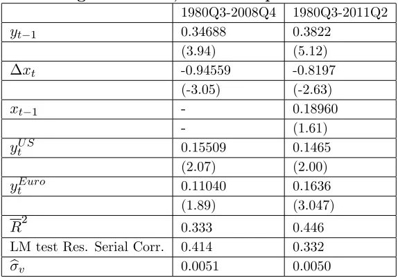
[image:22.612.159.446.311.512.2]and lagged spread, are shown in Table 1.
Table 1: ARDL in UK growth (y) and spread (x) augmented with US and Euro area growth rates, t ratios in parentheses.
1980Q3-2008Q4 1980Q3-2011Q2
yt 1 0.34688 0.3822
(3.94) (5.12)
xt -0.94559 -0.8197
(-3.05) (-2.63)
xt 1 - 0.18960
- (1.61)
yU S
t 0.15509 0.1465
(2.07) (2.00)
ytEuro 0.11040 0.1636
(1.89) (3.047)
R2 0.333 0.446
LM test Res. Serial Corr. 0.414 0.332
bv 0.0051 0.0050
The model indicates that a permanent 100 basis points reduction in the spread increases
predicted growth by almost 1% on impact, although this e¤ect is quickly reversed and disappears
altogether within two years. Although they do not emphasise this feature, the estimates of
Kapetanios et al. (2012), tell very much the same story: the bene…cial e¤ects of QE on growth are
of a similar size and rather short-lived. However this predicted positive e¤ect on growth of reducing
the spread is small relative to the large negative equation errors, the estimated equation
over-predicts growth during the recession. So the actual is below the counterfactual outcome without
QE in all but one post-intervention quarter. For H = 10; (2009Q1 2011Q2); d^H = 0:00315;
and from Table 1, ^0 = 0:347and ^0v = 0:0051:So the test statistic (44)
Td;Ha =
p
Hd^H
^0v
0
H^0H^0H H0 H
is 1:17:
The smallHadjustment used in (44) does not make very much di¤erence and the test statistic without it (47)
Td;Hb =
1 ^0 pHd^H
^0v
;
is 1:28. Also taking account of the sampling uncertainty associated with parameter estimation, captured by the second term in the denominator of (43), namely
(T H) 1 H0 ^0(1) T 1Q(0)Q0(0) 1
^00
(1) H0 >0;
will not alter the test outcome. Firstly, withT = 114 this second term is likely to be small, and secondly given that it is positive its inclusion can only reduce the statistical signi…cance of the
test.
As a result we can safely conclude that given our model speci…cation, the null that the QE
policy intervention was ine¤ective cannot be rejected. But at the same time we need to bear in
mind that, as with all statistical tests, the null hypothesis being tested is a joint null, assuming
that under the null hypothesis either no other major policy changes were put into e¤ect, or such
additional policy changes were also ine¤ective. Separating the e¤ects of QE from other policy
de-velopments, such as the austerity measures that were put into e¤ect by the Coalition Government
in the UK would be di¢ cult. However, since the austerity measures were not introduced till after
2010Q2, the joint null problem might not be that serious in the present application.
5
Conclusion
In this paper we have derived tests for the null hypothesis of the ine¤ectiveness of a policy
intervention, de…ned as a change in the parameters of a policy rule for reduced form policy
response equations, which are simpler to implement and could be more robust than the tests
based on possibly misspeci…ed complete structural models. In such cases we propose estimating
an unrestricted reduced form policy equation which makes the target variable a function of lagged
values of the target variable, as well as current and lagged values of the policy and policy-invariant
exogenous variables (if any).
The tests are based on the di¤erences, over a given policy evaluation horizon, between the
post-intervention realizations of the target variable and the associated counterfactual outcomes
based on the parameters estimated using data before the policy intervention. The Lucas Critique
is not an issue since the counterfactual, given by the predictions from the model estimated on
outcomes will embody any e¤ect of the change in policy, the change in parameters and the
conse-quent change in expectations. The tests do not require knowing the post-intervention parameters.
We derive the asymptotic distribution of the policy ine¤ectiveness tests under alternative
assumptions concerning the type of model, the future error processes and the pre and
post-intervention sample sizes. We also develop a policy ine¤ectiveness test based on the mean policy
e¤ect which is robust to the distribution of future errors, but requires the post-intervention, policy
evaluation horizon to be reasonably large. In the case of a static model we also derive an exact
test allowing for the estimation uncertainty.
We illustrate some of the issues that arise in counterfactual policy evaluation with an empirical
application to Quantitative Easing which was introduced in the UK in March 2009. The UK QE
involved exchanging one liability of the state - government bonds (gilts) - for another - claims
on the central bank. That change in the quantities of the two assets would cause a rise in the
price of guilts, decline in their yields, but also cause a rise in the prices of substitute assets such
as corporate bonds and equities. We estimate models explaining UK output growth over two
sample periods, one ending in 2008Q4 (before QE), and the other ending in 2011Q2. We use an
ARDL(1,1) between growth and the change in the spread of long government interest rates over
short rates, augmented by current values of US and euro area output growth. We follow the Bank
of England in assuming that QE caused a permanent 100 basis points reduction in the spread of
long interest rates over short interest rates after March 2009. The model indicates that QE had
an immediate positive e¤ect on growth, but this e¤ect tends to disappear quite quickly, certainly
within a year. The estimates of Kapetanios et al. (2012) for the time pro…les of the e¤ects of
the QE tell very much the same story, namely the bene…cial e¤ects of QE are rather short-lived.
We then apply the tests we have suggested and the null hypothesis of policy ine¤ectiveness is not
rejected. QE did not have a signi…cant e¤ect on UK growth.
References
Abadie, A., and J. Gardeazabal (2003): The Economic cost of con‡ict a case study of the
Basque country, American Economic Review,93, 113-132.
Angrist, J. D., and G. Kuersteiner (2011): Causal e¤ects of monetary policy shocks:
semipara-metric conditional independence tests with a multinomial propensity score,Review of Economics and Statistics, 93, 725-747.
Angrist, J. D., O. Jorda and G. Kuersteiner (2013): Semiparametric estimates of monetary
policy e¤ects: string theory revisited, NBER Working Paper No. 19355.
estimating the macroeconomic e¤ects of spread compression at the zero lower bound,International Journal of Central Banking, 9, 165-212.
Borio, C., and P. Disayatat (2010): Unconventional monetary policies: an appraisal,Manchester School, Supplement, 53-89.
Bowman, D., F. Cai, S. Davies and S. Kamin (2011): Quantitative Easing and Bank Lending:
evidence from Japan, Board of Governors of the Federal Reserve System, International Finance
Discussion Papers No. 1018.
Dees, S., F. di Mauro, M. H. Pesaran, and L. V. Smith (2007): Exploring the international
linkages of the euro area: a global VAR analysis, Journal of Applied Econometrics, 22, 1-38. Fagan, G., J. R. Lothian and P. D. McNelis (2013): Was the Gold Standard really Destabilising
Journal of Applied Econometrics 28, 231-249.
Fogel, R. W. (1964): Railroads and American Economic Growth, Johns Hopkins Press, Balti-more.
Giannone, D., M. Lenza, H. Pill and L. Reichlin (2011): Non-standard monetary policy
mea-sures and monetary developments, ECB Working Paper No. 1290.
Goodhart, C. A. E., and J. P. Ashworth (2012): QE: A successful start may be running into
diminishing returns,Oxford Review of Economic Policy 28, 640-670.
Hsiao, C., H. S. Ching and S. K. Wan (2012): A panel data approach for program evaluation:
measuring the bene…ts of political and economic integration of Hong kong with mainland China.
Journal of Applied Econometrics, 27, 705-740.
Imbens, G, and J. M. Wooldridge (2009): Recent developments in the econometrics of program
evaluation,Journal of Economic Literature, 47, 5-86.
Jorda, O., and A. M. Taylor (2013): The time for austerity: estimating the average treatment
e¤ect of …scal policy, NBER Working Paper No. 19414.
Joyce, M. A. S., A. Lasaosa, I. Stevens and M. Tong (2011): The …nancial market impact of
Quantitative Easing in the UK,International Journal of Central Banking, 7, 113-161.
Joyce, M. A. S., D. Miles, A. Scott and D. Vayanos (2012): Quantitative Easing and
Uncon-ventional Monetary Policy - An Introduction, Economic Journal, 122, F271-F288.
Kapetanios, G., H. Mumtaz, I. Stevens and K. Theodoridis (2012): Assessing the economy
wide e¤ects of quantitative easing, Economic Journal, 122, F316-347. Lewis, D. (1973): Counterfactuals, Blackwells, Oxford.
Meaning, J., and F. Zhu (2011): The impact of recent central bank asset purchase programs,
BIS Quarterly Review, December, 73-83.
Pesaran, M. H., A. Pick, and M. Pranovich (2013): Optimal forecasts in the presence of
structural breaks, Journal of Econometrics, 177, 134–152.
Pesaran, M.H., and Y. Shin (1999): An autoregressive distributed-lag modelling approach to
cointegration analysis, in (ed) S Strom, Econometrics and Economic Theory in the 20th Century: The Ragnar Frisch Centennial Symposium, 1999, Chapter 11, pp. 371-413. Cambridge University Press, Cambridge.
Pesaran, M. H., L. V. Smith and R. P. Smith (2007): What if the UK or Sweden had joined
the euro in 1999? An empirical evaluation using a Global VAR.International Journal of Finance and Economics, 12, 55-87.
Pesaran, M.H. and R. P Smith, (2014a), Signs of Impact E¤ects in Time Series Regression
Models,Economics Letters, 122, 150-153.
Pesaran, M.H. and R.P. Smith (2014b) Tests of Policy Ine¤ectiveness in Macroeconometrics,
USC Center for Applied Financial Economics, CAFE Research Paper No. 14.07.
Zellner, A., and F. Palm (1974), Time series analysis and simultaneous equation econometric
models, inThe Structural Econometric Time Series Analysis Approach, edited by A. Zellner and F.C. Palm,Cambridge University Press, Cambridge.
Appendices
Appendix A1: Derivation of the distribution of Fd;H de…ned by (24)
Under the null hypothesis Hs0 de…ned by (20) ^
d(1) =v(1) S0(1) S0(0)S(0) 1
S0(0)v(0) =G0v;
y(0) S(0)^0ys= IT S(0) S0(0)S(0) 1
S(0) v(0)=Qv;
wherev= (v0(0);v0(1))0, and
G0 = S0(1) S0(0)S(0) 1
S0(0); IH ;
Q= IT S(0) S0(0)S(0) 1
S(0) 0T H
0H T 0H H !
:
Using these results inFd;H de…ned by (24), we have
Fd;H=
T kx kw
H
^
d0(1) IH +S0(1) S0(0)S(0) 1
S0(1)0 1
^ d(1)
v0(0) IH S(0) S0(0)S(0) 1
S(0) v(0)
= T kx kw
H
0G(G0G) 1G0
where =v= 0v s N(0;IT+H). It is also easily seen that G(G0G) 1G0and Q are idempotent
matrices that are orthogonal (namely,G0Q=0) with ranksH and T kx kw, which establish
thatFd;H has a F distribution withH and T kx kw degrees of freedom.
Appendix A2: Derivation of the distribution of Td;H in the general dynamic case
Consider the general ARDL speci…cation given by (28) and (29). In this case, setting py =p
to simplify the notation, the post-intervention model can be written as
1
Hy(1) = 1Hyp+S(1) 1ys+v(1);
whereypis theH 1vector containing thepinitial observations,yp = (yT0; yT0 1; :::; yT0 p+1;0; :::;0)0;
1 H = (
1), 1
H = H( 1); = ( 1: 2; :::; p)0,
H( ) = 0 B B B B B B B B B B B B B B @
1 0 0 0 0 0 0 0
1 1 0 0 0 0 0 0
2 1 1 0 0 0 0 0
..
. ... ... ... 0 0 0 0
p p 1 1 0 0 0 0
0 0 0 0 0 0 0
..
. ... ... ... ... ... ... ...
0 0 p p 1 1 0
0 0 0 p 1 1
1 C C C C C C C C C C C C C C A
H( ) = 0 B B B B B B B B B B @
1 2 0 p
2 3 p 0
..
. ... ... ...
p 0 0 0
0 0 0 0
..
. ... ... ...
0 0 0 0
1 C C C C C C C C C C A ;
and as before,S(1) represents theH kmatrix of post-intervention observations on the exogenous
variables,xt and wt, and their lagged values,k= (1 +px)kx+ (1 +pw)kw. Also
1
H ( ) = H( ) = 0 B B B B B @
a0 0 0 0 0
a1 a0 0 0 0
..
. ... ... ... ...
aH 2 aH 3 a0 0
aH 1 aH 2 a1 a0 1 C C C C C A ; (48)
where h is obtained recursively using the di¤erence equation
ah = p X
i=1
with a0 = 1 and ai = 0, for all i < 0. It is easily veri…ed that for p = 1, H( ) de…ned by
(48) reduces to the matrix de…ned by (33). Using the above set up, the estimated counterfactual
outcomes are given by
^
y0(1)= H(^0) h
H(^0)yp+X(1)0 ^yx0 +W(1)^0yw; i
= ^0H
h ^0
Hyp+S0(1)^ 0 ys
i
;
where '^0 = ^00;^ys00 0 is obtained estimating the ARDL regression using the pre-intervention sample. The mean policy ine¤ectiveness test can be de…ned as before,Td;H =
p
Hd^H=!^0, where
^
dH =H 1 H0 ^d(1);d^(1) =y(1) y^0(1),
^
!20 = ^20vhH 1 H0 H(^0) 0H(^0) H i
;
and ^2
0v is the estimate of 20v based on the pre policy sample. Following the same line of
rea-soning as in sub-section 3.2, it follows that Td;H !dN(0;1), under the null hypothesis of policy