http://dx.doi.org/10.4236/ojs.2015.51004
How to cite this paper: Onyeka, A.C., Izunobi, C.H. and Iwueze, I.S. (2015) Separate-Type Estimators for Estimating
Popula-Separate-Type Estimators for Estimating
Population Ratio in Post-Stratified Sampling
Using Variable Transformation
Aloy Chijioke Onyeka, Chinyeaka Hostensia Izunobi, Iheanyi Sylvester Iwueze Department of Statistics, Federal University of Technology, Owerri, Nigeria
Email: [email protected], [email protected], [email protected]
Received 7 January 2015; accepted 25 January 2015; published 30 January 2015
Copyright © 2015 by authors and Scientific Research Publishing Inc.
This work is licensed under the Creative Commons Attribution International License (CC BY). http://creativecommons.org/licenses/by/4.0/
Abstract
The study proposes, along the line of [1], six separate-type estimators for estimating the popula-tion ratio of two variables in post-stratified sampling, using variable transformapopula-tion. Properties of the proposed estimators were obtained up to first order approximations, both for achieved sam-ple configurations (conditional argument) and over repeated samsam-ples of fixed size n (uncondi-tional argument). Efficiency conditions, under which the proposed separate-type estimators would perform better than the associated customary separate-type estimators in terms of having smaller mean squared errors, were obtained. Furthermore, conditions under which some of the proposed separate-type estimators would perform better than other proposed separate-type estimators were also obtained. The optimum estimators among the proposed separate-type estimators were obtained and an empirical illustration confirmed the theoretical results.
Keywords
Variable Transformation, Separate-Type Estimator, Optimum Estimators, Ratio, Product and Regression-Type Estimators, Mean Squared Error
1. Introduction
Information on auxiliary character has been used by many authors [2]-[9] in sample survey to improve estimates of population parameters of the study variable, and sometimes, information on several variables is used to esti-mate or predict a characteristic of interest, such as mean, total, ratio, and proportion. Reference [1] proposed the following six (6) estimators of the population ratio
(
R=Y X)
of the population means of two variables, y(
)
(
)
1
ˆ y regression-type estimator of sample mean,
R x
x b x∗ X
=
− − (1.1)
(
)
2
ˆ y yx ratio-type estimator of sample mean,
R x
x xX X x
∗
∗
= =
(1.2)
(
)
3
ˆ y yX product-type estimator of sample mean,
R x
xx xx
X
∗ ∗
= =
(1.3)
(
)
4
ˆ y transformed mean estimator,
R x
x
∗ ∗
= (1.4)
(
)
(
)
5
ˆ y regression-type estimator of transformed mean,
R x
x b x X
∗ ∗
=
− − (1.5)
(
)
6
ˆ y yx ratio-type estimator of transformed mean,
R x
x X x
X x
∗ ∗
∗
= =
(1.6)
where, y, x and x∗ are sample means of the variables yi, xi and xi
∗
respectively,
, 1, 2, ,
i i
NX nx
x i N
N n
∗ = − =
− (1.7)
(
1)
, nx X x
N n
π π π
∗= + − =
− (1.8) and b is a suitable constant, often chosen to be very close to the population regression coefficient of y on x. Reference [1] noted that authors like [8] [10]-[14] had used the variable transformation (1.7) or its equiva-lence in their respective studies. The obvious advantage of variable transformation is the introduction of an ad-ditional auxiliary (transformed) variable without adad-ditional cost, since the new auxiliary variable is a transfor-mation of an already observed auxiliary variable. The work carried out by [1] was restricted to simple random sampling scheme. The present study extends the work carried out by [1] to post-stratified random sampling, by considering six (6) separate-type estimators of the population ratio of two variables in post-stratified random sampling, proposed along the line of the estimators proposed by [1] under the simple random sampling scheme.
2. The Proposed Separate-Type Estimators
Let n units be drawn from a population of N units using simple random sampling method and let the sam-pled units be allocated to their respective strata, where nh is the number of units that fall into stratum h such
that
1
L h h
n n
= =
∑
. Let yhi and xhi be theth
i observation on the study and auxiliary variables. Consider the
following variable transformation of the auxiliary variable, x, under post-stratified sampling scheme.
, 1,2, , and 1, 2, ,
hi hi
NX nx
x h L i N
N n
∗ = − = =
− (2.1)
with the associated sample mean
(
1)
whereps ps
n
x X x
N n
π π π
∗ = − − =
− (2.2)
where
1
L ps h h
h
x ω x
=
=
∑
and1
L ps h h
h
y ω y
=
∑
are sample mean estimators based on xhi and yhi respectively.Using the sample means yps, xps and xps
∗
va-riable x, is known, we proposed six separate-type estimators of the population ratio R=Y X in post strati-fied sampling scheme, following [1], as
(
)
1 1
ˆ L h
S h
h h h h
y R
x b x X
ω ∗
=
=
− −
∑
(2.3)2
1 1
ˆ L h L h h
S h h
h h h h h
h h
y y x R
x X x
X x
ω ω ∗
= =
∗
= =
∑
∑
(2.4)3
1 1
ˆ L h L h h
S h h
h h h h h h
h
y y X R
x x x x
X
ω ∗ ω ∗
= =
= =
∑
∑
(2.5)4 1
ˆ L h
S h h h
y R
x
ω ∗
=
=
∑
(2.6)(
)
5 1
ˆ L h
S h
h h h h
y R
x b x X
ω ∗
=
=
− −
∑
(2.7)6
1 1
ˆ L h L h h .
S h h
h h h h h
h h
y y x R
x X x
X x
ω ∗ ω ∗
= =
= =
∑
∑
(2.8)2.1. The Conditional Properties of the Proposed Separate-Type Estimators Let
0 and 1 .
h h h h
h h
h h
y Y x X
e e
Y X
− −
= = (2.9)
Then under the conditional argument,
( )
( )
2 0h 1h 0
E e =E e = (2.10)
( )
2 2( )
(
)
22 1 2 2
1 1
h xh
h h
h
h h
V x S
E e f
n X X
= = − (2.11)
( )
2 2( )
(
)
22 1 2 2
1 1
h xh
h h
h
h h
V x S
E e f
n X X
= = − (2.12)
(
)
2(
)
(
)
2 0 1
, 1
1 yxh
h h
h h h
h h h h h
S C y x
E e e f
Y X Y X n
= = − (2.13)
where E2 refers to conditional expectation. Notice that the first proposed estimator (2.3) can be rewritten as
1 1
1
ˆ L ˆ
S h h h
R ω R
=
=
∑
(2.14)where
(
)
1
ˆ h
h
h h h
y R
x b x∗ X
=
− − (2.15)
such that expanding up to first order approximation,
( )
1o n− , in expected value, we obtain
(
)
(
(
)
(
)
(
)
2 2)
1 0 1 0 1 1
ˆ 1 1 1
h h h h h h h h
and
(
)
2(
(
)
2(
)
)
2 2 2
1 0 1 0 1
ˆ 1 2 1 .
h h h h h h h
R −R =R e + +bπ e − +bπ e e (2.17)
We take conditional expectation of (2.16) and (2.17) and use (2.10) to (2.13) to make the necessary substitu-tions to obtain the conditional bias and mean square error of Rˆ1h respectively as
( )
(
)
(
)
2 2(
)
2 1 2
1 1
ˆ h 1 1
h h xh yxh
h h
f
B R R b S b S
n X π π
−
= + − + (2.18)
and
( )
(
)
2(
)
2 2 2(
)
2 1 2
1 1
ˆ
MSE h h yh 1 h xh 2 1 h yxh
h h
f
R S b R S b R S
n X π π
−
= + + − + (2.19)
so that, using (2.14)
( )
( )
(
)
(
)
2 2(
)
2 1 2 1 2
1 1
1 1
ˆ L ˆ L h 1 1
S h h h h xh yxh
h h h h
f
B R B R R b S b S
n X
ω ω π π
= =
−
=
∑
=∑
+ − + (2.20)and
( )
2( )
2(
)
2(
)
2 2 2(
)
2 1 2 1 2
1 1
1 1
ˆ ˆ
MSE 1 2 1 .
L L
h
S h h h yh h xh h yxh
h h h h
f
R B R S b R S b R S
n X
ω ω π π
= =
−
=
∑
=∑
+ + − + (2.21)Following similar procedure, we obtain the conditional biases and mean square errors of the six proposed
separate-type estimators, together with those of the customary separate-type estimator,
1
ˆ L h
S h h h y R x ω =
=
∑
, of popu-lation ratio
( )
R in post-stratified sampling, up to first order approximation as:( )
(
)
22 2
1
1 1
ˆ L h
S h h xh yxh
h h h
f
B R R S S
n X
ω
=
−
=
∑
− (2.22)( )
(
)
(
)
2 2(
)
2 1 2
1
1 1
ˆ L h 1 1
S h h xh yxh
h h h
f
B R b R S b S
n X
ω π π
=
−
=
∑
+ − + (2.23)( )
(
)
(
)
2(
)
2 2 2
1
1 1
ˆ L h 1 1
S h h xh yxh
h h h
f
B R R S S
n X
ω π π
=
−
=
∑
+ − + (2.24)( )
(
)
(
2)
2(
)
2 3 2
1
1 1
ˆ L h 1 1
S h h xh yxh
h h h
f
B R R S S
n X
ω π π π
=
−
=
∑
− + − − (2.25)( )
(
)
2 22 4 2
1
1 1
ˆ L h
S h h xh yxh
h h h
f
B R R S S
n X
ω π π
=
−
=
∑
+ (2.26)( )
(
)
(
)
2 2(
)
2 5 2
1
1 1
ˆ L h
S h h xh yxh
h h h
f
B R b R S b S
n X
ω π π
=
−
=
∑
+ + + (2.27)( )
(
)
(
)
2(
)
2 6 2
1
1 1
ˆ L h 1 1
S h h xh yxh
h h h
f
B R R S S
n X
ω π π π
=
−
=
∑
+ + + (2.28)and,
( )
2(
)
2 2 22 2 1 1 1 ˆ MSE 2 L h
S h yh h xh h yxh
h h h
f
R S R S R S
n X
ω
=
−
=
∑
+ − (2.29)( )
2(
)
2(
)
2 2 2(
)
2 1 2
1
1 1
ˆ
MSE 1 2 1
L
h
S h yh h xh h yxh
h h h
f
R S b R S b R S
n X
ω π π
=
−
( )
2(
)
2(
)
2 2 2(
)
2 2 2
1
1 1
ˆ
MSE 1 2 1
L
h
S h yh h xh h yxh
h h h
f
R S R S R S
n X
ω π π
=
−
=
∑
+ + − + (2.31)( )
2(
)
2(
)
2 2 2(
)
22 3 2
1
1 1
ˆ
MSE 1 2 1
L
h
S h yh h xh h yxh
h h h
f
R S R S R S
n X
ω π π
=
−
=
∑
+ − − − (2.32)( )
2(
)
2 2 2 22 4 2
1 1 1 ˆ MSE 2 L h
S h yh h xh h yxh
h h h
f
R S R S R S
n X
ω π π
=
−
=
∑
+ + (2.33)( )
2(
)
2(
)
2 2 2(
)
2 5 2
1 1 1 ˆ MSE 2 L h
S h yh h xh h yxh
h h h
f
R S b R S b R S n X
ω π π
=
−
=
∑
+ + + + (2.34)( )
2(
)
2(
)
2 2 2(
)
2 6 2
1
1 1
ˆ
MSE 1 2 1 .
L
h
S h yh h xh h yxh
h h h
f
R S R S R S
n X
ω π π
=
−
=
∑
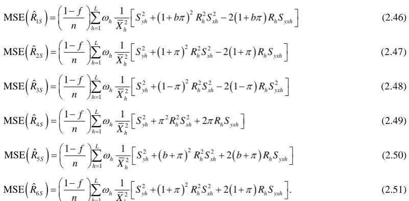
+ + + + (2.35)Generally, the conditional mean square errors of the proposed separate-type estimators are obtained as:
( )
2(
)
2 2 2 22 2 1 1 1 ˆ MSE 2 L h
qS h yh q h xh q h yxh
h h h
f
R S R S R S
n X
ω θ θ
=
−
=
∑
+ − (2.36)where q=1,, 6 and
(
)
(
)
(
)
(
)
(
)
1 1 b , 2 1 , 3 1 , 4 , 5 b , 6 1 .
θ = + π θ = +π θ = −π θ = −π θ = − π+ θ = − +π (2.37)
2.2. The Unconditional Properties of the Proposed Separate-Type Estimators
We take unconditional expectation of the conditional biases and mean square errors of (2.22) to (2.37) to obtain the unconditional properties of the separate type estimators as:
( )
22 1
1 1
ˆ L h
S h h xh yxh
h h h
f
B R R S S
n X ω = − = −
∑
(2.38)( )
(
)
2 2(
)
1 2
1
1 1
ˆ L h 1 1
S h h xh yxh
h h h
f
B R b R S b S
n X
ω π π
=
−
= + − +
∑
(2.39)( )
(
)
2(
)
2 2
1
1 1
ˆ L h 1 1
S h h xh yxh
h h h
f
B R R S S
n X
ω π π
=
−
= + − +
∑
(2.40)( )
(
2)
2(
)
3 2
1
1 1
ˆ L h 1 1
S h h xh yxh
h h h
f
B R R S S
n X
ω π π π
=
−
= − + − −
∑
(2.41)( )
2 24 2
1
1 1
ˆ L h
S h h xh yxh
h h h
f
B R R S S
n X
ω π π
=
−
= +
∑
(2.42)( )
(
)
2 2(
)
5 2
1
1 1
ˆ L h
S h h xh yxh
h h h
f
B R b R S b S
n X
ω π π
=
−
= + + +
∑
(2.43)( )
(
)
2(
)
6 2
1
1 1
ˆ L h 1 1
S h h xh yxh
h h h
f
B R R S S
n X
ω π π π
=
−
= + + +
∑
(2.44)and,
( )
2 2 22 1 1 1 ˆ MSE 2 L
S h yh h xh h yxh h h
f
R S R S R S
n =ω X
−
= + −
( )
2(
)
2 2 2(
)
1 2
1
1 1
ˆ
MSE 1 2 1
L
S h yh h xh h yxh
h h
f
R S b R S b R S
n =ω X π π
−
= + + − +
∑
(2.46)( )
2(
)
2 2 2(
)
2 2
1
1 1
ˆ
MSE 1 2 1
L
S h yh h xh h yxh h h
f
R S R S R S
n =ω X π π
−
= + + − +
∑
(2.47)( )
2(
)
2 2 2(
)
23 2
1
1 1
ˆ
MSE 1 2 1
L
S h yh h xh h yxh h h
f
R S R S R S
n =ω X π π
−
= + − − −
∑
(2.48)( )
2 2 2 24 2 1 1 1 ˆ MSE 2 L
S h yh h xh h yxh h h
f
R S R S R S
n = ω X π π
−
= + +
∑
(2.49)( )
2(
)
2 2 2(
)
5 2 1 1 1 ˆ MSE 2 L
S h yh h xh h yxh h h
f
R S b R S b R S
n =ω X π π
−
= + + + +
∑
(2.50)( )
2(
)
2 2 2(
)
6 2
1
1 1
ˆ
MSE 1 2 1 .
L
S h yh h xh h yxh h h
f
R S R S R S
n =ω X π π
−
= + + + +
∑
(2.51)Generally, the unconditional mean square errors of the proposed separate-type estimators of the population ratio are obtained as:
( )
2 2 2 22 1
1 1
ˆ
MSE 2 .
L
qs h yh q h xh q h yxh h h
f
R S R S R S
n = ω X θ θ
−
= + −
∑
(2.52)3. Efficiency Comparison
The efficiencies of the six proposed separate-type estimators, ˆRqs, were first compared with that of the
custo-mary separate-type estimator Rˆs in estimating the population ratio, R, of two population means under the conditional and unconditional arguments in post stratified random sampling scheme. Secondly, the perfor-mances of the proposed estimators among themselves were also compared, and finally, the optimum estimators among the proposed estimators were obtained. The efficiency conditions were based on estimators with smaller mean squared errors, and the results are shown inTable 1.
4. Numerical Illustration
[image:6.595.140.541.82.279.2]Here, we use the final year GPA
( )
y and the level of absenteeism( )
x of 2012/2013 graduating students of Statistics department, Federal University of Technology Owerri to illustrate the properties of the estimators proposed in the present study. Absenteeism is the average number of days absent from lectures in a month. TheTable 1. Efficiency conditions under the conditional and unconditional arguments.
Estimator Conditional argument Unconditional argument
qs
R is better than Rs if:
1) 1 and 1 or
2) 1 and 1
q q θ β θ β ′′ < < ′′
> >
1) 1 and 1 or
2) 1 and 1
q q θ β θ β ∗ ∗ < <
> >
js
R is better than Rks if:
1) and or
2) and
j k j
j k j
θ θ θ β
θ θ θ β
′′ < < ′′
> >
1) and or
2) and
j k j
j k j
θ θ θ β
θ θ θ β
∗ ∗ < <
> >
qs
R is optimum if: 0
q
θ =β′′ 0
q
θ =β∗
Where ( ) ( ) 2 2 1
2 2 2 2 1
1
1
L
h h yxh h
h h h
L
h h xh h
h h h
f S R n X
f S R n X
ω
β = ω
= − ′′ = −
∑
∑
, 2 1 2 2 2 1 L h h yxhh h
L h h xh
h h R S X R S X ω
β∗ = ω
=
=
∑
class consists of 50 students, with 32 and 18 students respectively falling into low-absenteeism (0 - 3 days per month) and high-absenteeism (4 - 6 days per month) groups or strata. Our interest is to estimate the ratio of final year GPA to absenteeism from lectures, based on a post-stratified sample of 20 out of the 50 students in the class. The data statistics, consisting mainly of population parameters, are shown inTable 2.
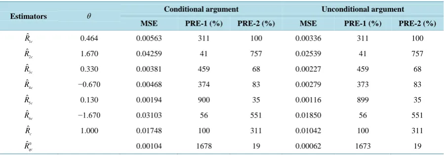
Table 3 shows the percentage relative efficiencies (PRE-1) of the proposed separate-type estimators, ˆRqs,
over the customary separate-type estimator, Rˆs, under the conditional argument and unconditional arguments. The table also shows the percentage relative efficiency (PRE-2) of one of the proposed separate-type estimators,
1
ˆ s
[image:7.595.89.539.561.718.2]R , over the other separate-type estimators, under the conditional and unconditional arguments.
Table 3 shows that apart from the estimators, Rˆ2s and Rˆ6s, the remaining four proposed separate-type es-timators, under the conditional and unconditional arguments, are more efficient than the customary separate-type estimator, Rˆs, for the data under consideration, and their gains in efficiency (PRE-1) are relatively large. Also, using, PRE-2 we observe that the proposed separate-type estimator, Rˆ1s, is more efficient than the estimators,
2
ˆ s
R , Rˆ6s, and Rˆs, under the conditional argument and unconditional arguments. The optimum estimator, as expected, has the highest gain in efficiency. However, the customary separate-type estimator is found to be more efficient than some of the proposed separate-type estimators for the given data set. This confirms the theoretical results which shows that the proposed estimators are not always more efficient than the customary separate es-timators. Hence, the empirical results confirm the theoretical results.
5. Concluding Remarks
The present study extended the use of variable transformation in estimating population ratio in simple random
Table 2. Data statistics for final year GPA (y) and absenteeism from lectures (x).
Population/sample parameters
Stratum 1 (low-absenteeism)
Stratum 2 (high-absenteeism)
50
N= N1=32 N2=18
20
n= n1=12 n2=8
(1−f)=0.60 (1−f1)=0.625 (1−f2)=0.556
2.98
Y= Y1=3.16 Y2=2.65
3.16
X= X1=2.03 X2=5.17
0.94
R= R1=1.56 R2=0.51
0.67
π= 2
1 0.2422
y
S = 2
2 0.0389
y
S =
0.80
b= − 2
1 0.9990
x
S = 2
2 0.6176
x
S =
1 0.2124
yx
S = − Syx2= −0.0161
1 0.64
ω = ω =2 0.36
Table 3. Efficiency comparison of proposed separate-type estimators.
Estimators θ Conditional argument Unconditional argument
MSE PRE-1 (%) PRE-2 (%) MSE PRE-1 (%) PRE-2 (%)
1
ˆ
c
R 0.464 0.00563 311 100 0.00336 311 100
2
ˆ
c
R 1.670 0.04259 41 757 0.02539 41 757
3
ˆ
c
R 0.330 0.00381 459 68 0.00227 459 68
4
ˆ
c
R −0.670 0.00468 374 83 0.00279 373 83
5
ˆ
c
R 0.130 0.00194 900 35 0.00116 899 35
6
ˆ
c
R −1.670 0.03103 56 551 0.01850 56 551
ˆ
c
R 1.000 0.01748 100 311 0.01042 100 311
0
ˆ
qc
sampling scheme to post-stratified sampling scheme where we proposed six separate-type estimators. Efficiency conditions under which the proposed estimators performed better than the customary separate-type estimators were obtained. Both the theoretical and empirical comparisons show that the proposed estimators are not always better or more efficient than the customary separate-type estimator of the population ratio in post-stratified sam-pling. Consequently, in any given survey, these efficiency conditions should be employed to determine the ap-propriate separate-type estimators to use for estimating the population ratio of two variables in post-stratified sampling scheme using variable transformation. The major advantage of the proposed estimators is the use of additional (transformed) auxiliary variable without additional cost, since the additional auxiliary variable is a transformation of an already observed auxiliary variable.
References
[1] Onyeka, A.C., Nlebedim, V.U. and Izunobi, C.H. (2013) Estimation of Population Ratio in Simple Random Sampling Using Variable Transformation. Global Journal of Science Frontier Research, 13, 57-65.
[2] Cochran, W.G. (1940) The Estimation of the Yields of the Cereal Experiments by Sampling for the Ratio of Grain to Total Produce. The Journal of Agricultural Science, 30, 262-275. http://dx.doi.org/10.1017/S0021859600048012 [3] Robson, D.S. (1957) Application of Multivariate Polykays to the Theory of Unbiased Ratio-Type Estimation. Journal
of the American Statistical Association, 52, 511-522. http://dx.doi.org/10.1080/01621459.1957.10501407
[4] Murthy, M.N. (1964) Product Method of Estimation. Sankhya, Series A, 26, 294-307.
[5] Singh, M.P. (1965) On the Estimation of Ratio and Product of the Population Parameters. Sankhya, Series B, 27, 321- 328.
[6] Sukhatme, P.V. and Sukhatme, B.V. (1970) Sampling Theory of Surveys with Applications. Iowa State University Press, Ames.
[7] Cochran, W.G. (1977) Sampling Techniques. 3rd Edition, John Wiley & Sons, New York.
[8] Onyeka, A.C. (2013) Dual to Ratio Estimators of Population Mean in Post-Stratified Sampling Using Known Value of Some Population Parameters. Global Journal of Science Frontier Research, 13, 13-23.
[9] Onyeka, A.C., Nlebedim, V.U. and Izunobi, C.H. (2014) A Class of Estimators for Population Ratio in Simple Random Sampling Using Variable Transformation. Open Journal of Statistics, 4, 284-291.
http://dx.doi.org/10.4236/ojs.2014.44029
[10] Srivenkataramana, T. (1980) A Dual of Ratio Estimator in Sample Surveys. Biometrika, 67, 199-204. http://dx.doi.org/10.1093/biomet/67.1.199
[11] Upadhyaya, L.N., Singh, G.N. and Singh, H.P. (2000) Use of Transformed Auxiliary Variable in the Estimation of Population Ratio in Sample Survey. Statistics in Transition, 4, 1019-1027.
[12] Singh, H.P. and Tailor, R. (2005) Estimation of Finite Population Mean Using Known Correlation Coefficient between Auxiliary Characters. Statistica, Anno LXV, 4, 407-418.
[13] Tailor, R. and Sharma, B.K. (2009) A Modified Ratio-Cum-Product Estimator of Finite Population Mean Using Known Coefficient of Variation and Coefficient of Kurtosis. Statistics in Transition—New Series, 10, 15-24.