Changes in Köppen Geiger climate types under a future climate for Australia: hydrological implications

www.hydrol-earth-syst-sci.net/16/3341/2012/ doi:10.5194/hess-16-3341-2012

© Author(s) 2012. CC Attribution 3.0 License.

Earth System

Sciences

Changes in K¨oppen-Geiger climate types under a future climate for

Australia: hydrological implications

R. S. Crosbie1, D. W. Pollock2,*, F. S. Mpelasoka3, O. V. Barron2, S. P. Charles2, and M. J. Donn2 1_{CSIRO Water for a Healthy Country National Research Flagship, CSIRO Land and Water, PMB 2,} Glen Osmond SA 5064, Australia

2_{CSIRO Water for a Healthy Country National Research Flagship, CSIRO Land and Water, Private Bag 5, Wembley,} WA 6913, Australia

3_{CSIRO Water for a Healthy Country National Research Flagship, CSIRO Land and Water, G.P.O. Box 1666,} Canberra ACT 2601, Australia

*_{now at: Rio Tinto Iron Ore, 152–158 St George’s Terrace Perth 6000, Western Australia}

Correspondence to: R. S. Crosbie ([email protected])

Received: 17 May 2012 – Published in Hydrol. Earth Syst. Sci. Discuss.: 12 June 2012 Revised: 29 August 2012 – Accepted: 29 August 2012 – Published: 18 September 2012

Abstract. The K¨oppen-Geiger climate classification has been used for over a century to delineate climate types across the globe. As it was developed to mimic the distribution of vegetation, it may provide a useful surrogate for making pro-jections of the future distribution of vegetation, and hence resultant hydrological implications, under climate change scenarios. This paper developed projections of the K¨oppen-Geiger climate types covering the Australian continent for a 2030 and 2050 climate relative to a 1990 historical baseline climate using 17 Global Climate Models (GCMs) and five global warming scenarios. At the highest level of classifica-tion for a +2.4◦C future climate (the upper limit projected for 2050) relative to the historical baseline, it was projected that the area of the continent covered by

– tropical climate types would increase from 8.8 % to 9.1 %;

– arid climate types would increase from 76.5 % to 81.7 %;

– temperate climate types would decrease from 14.7 % to 9.2 %;

– cold climate types would decrease from 0.016 % to 0.001 %.

Previous climate change impact studies on water resources in Australia have assumed a static vegetation distribution.

If the change in projected climate types is used as a sur-rogate for a change in vegetation, then the major transition in climate from temperate to arid in parts of Australia un-der a drier future climate could cause indirect effects on wa-ter resources. A transition from annual cropping to perennial grassland would have a compounding effect on the projected reduction in recharge. In contrast, a transition from forest to grassland would have a mitigating effect on the projected re-duction in runoff.

1 Introduction

The K¨oppen-Geiger climate classification (K¨oppen, 1936) is the most widely applied method for determining climate zones; it has been used recently in such diverse fields as environmental science, veterinary science and mathematics (Rubel and Kottek, 2011). Its origins can be traced to obser-vations of the distribution of vegetation throughout Russia (K¨oppen, 1884) and is still under active development (Kot-tek et al., 2006; Peel et al., 2007; Rubel and Kot(Kot-tek, 2010).

global biome model of Prentice et al. (1992). This link be-tween climate and vegetation is very useful because climate is more readily mapped than vegetation.

Vegetation also exerts a strong control over hydrology. Us-ing data from over 250 catchments around the world, Zhang et al. (2001) demonstrated that for any given annual average rainfall a forested catchment will have a higher evapotranspi-ration than a grassed catchment. Similarly, from a review of Australian field studies of groundwater recharge, Crosbie et al. (2010a) showed that for a given annual average rainfall groundwater recharge was highest under annual vegetation and lowest under tree type vegetation. Any change in vege-tation will have a corresponding impact upon the hydrology of a catchment.

Projections of water resources availability under a future climate have generally assumed a static vegetation cover-age, either implicitly through calibration of a rainfall-runoff model (Chiew et al., 2009b) or explicitly through having a pre-defined vegetation layer as an input to the modelling process (Crosbie et al., 2010b). The limitations of this as-sumption have been discussed (Holman et al., 2012; Holman, 2006), but there are few examples in the literature of the in-direct effects of climate change on water resources due to vegetation change (one such example is Holman, 2006). Pro-jections of changes in vegetation can be modelled in man-aged systems using coupled crop growth and economic mod-els (Holman, 2006) or in natural systems using dynamic veg-etation growth models (Cramer et al., 2001), however this adds complexity and computational demands upon studies investigating the climate change impacts on water resources. Given that the K¨oppen-Geiger climate classification was developed to mimic the distribution of vegetation types (K¨oppen, 1884), it may provide a relatively simple surrogate for providing projections of future vegetation types under cli-mate change scenarios (Kleidon et al., 2000). This paper aims to investigate the changes in climate types for Australia un-der a future climate based upon projections from an ensem-ble of global climate models (GCMs) and a range of global warming scenarios and then to discuss the hydrological im-plications of the projected change in climate types.

2 Methods

The K¨oppen-Geiger classification is calculated from long term averages of temperature and precipitation at an an-nual, seasonal and monthly time scale. For the definitions described by Peel et al. (2007), there are 30 discrete cli-mate types, 15 of which are present in Australia (Table 1). At the highest level there are five climate types: tropical (A), arid (B), temperate (C), cold (D) and polar (E). Within these five top level climate types there are a number of further classes with a second level and third level delineated by met-rics derived from monthly rainfall and temperature. For a full description of the classification criteria, the reader is referred to Peel et al. (2007).

For this study, the historical climate data used as inputs for calculating the distribution of the K¨oppen-Geiger cli-mate types across Australia came from the monthly gridded (0.05◦) climate surfaces of the Bureau of Meteorology (Jones et al., 2009). These are created by interpolation of rainfall and temperature anomalies from observation data relative to the period 1971–2000, for the year 1990 this included over 6000 rainfall stations and 600 temperature stations (Jones et al., 2009).

The historical time period considered by this study is 1970 to 2010, this is 20 years either side of a 1990 centred base-line climate. The future climate scenarios are defined by global warming above a 1990 climate. We have considered a low, medium and high global warming scenario for 2030 (+0.7◦C, +1.0◦C and +1.3◦C) and 2050 (+1.0◦C, +1.7◦C and +2.4◦_{C) based upon previous work (Crosbie et al., 2012;}

Post et al., 2012) that inferred the degree of global warming from the IPCC Fourth Assessment Report (IPCC, 2007; Na-kicenovic and Swart, 2000). These levels of global warming can be considered a surrogate for time, in that the +2.4◦C used here as the high global warming scenario for 2050 could equally be considered a very low global warming scenario for 2100.

For the future climate scenarios the outputs of the GCMs had to be downscaled from the coarse grid of the GCMs (>1◦) to the fine grid of the historical climate data (0.05◦), downscaling is also necessary to remove the bias from the GCM data (Fowler et al., 2007). The future climate output from 17 GCMs (Table 2) that are archived by the World Cli-mate Research Programme’s (WCRP’s) Coupled Model In-tercomparison Project phase 3 (CMIP3) multi-model dataset (Meehl et al., 2007) were used to derive monthly scaling fac-tors as a percentage change in rainfall per degree of global warming and a change in temperature per degree of global warming at the grid resultion of each GCM (Mitchell, 2003; Mpelasoka and Chiew, 2009; Suppiah et al., 2007). These scaling factors were applied to the observed time series of historical monthly gridded rainfall and temperature to cre-ate projections for the five global warming scenarios (the +1.0◦C is used for both 2030 and 2050) for each of the 17 GCMs. These 85 future climate variants were then assessed on a gridded basis to determine the projected future distribu-tion of K¨oppen-Geiger climate types across Australia using the definitions of Peel et al. (2007). To simplify the results, the mode of the K¨oppen-Geiger climate types derived from the 17 GCMs has been reported for each of the five global warming scenarios.

Table 1. Description of the K¨oppen-Geiger climate types in

Aus-tralia, see Peel et al. (2007) for classification criteria.

Code Description Af Tropical, Rainforest Am Tropical, Monsoon Aw Tropical, Savannah BWh Arid, Desert, Hot BWk Arid, Desert, Cold BSh Arid, Steppe, Hot BSk Arid, Steppe, Cold

Csa Temperate, Dry Summer, Hot Summer Csb Temperate, Dry Summer, Warm Summer Cwa Temperate, Dry Winter, Hot Summer Cfa Temperate, Without dry season, Hot Summer Cfb Temperate, Without dry season, Warm Summer Cfc Temperate, Without dry season, Cold Summer Dfb Cold, Without dry season, Warm Summer Dfc Cold, Without dry season, Cold Summer

3 Results

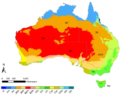
The historical baseline climate types derived from this study are different from those produced by Peel et al. (2007) and Kottek et al. (2006) due to differences in the input data. Jones et al. (2009) had access to more than three times as many rainfall stations and more than twice as many temperature stations compared to Peel et al. (2007) to create the gridded climate surfaces used here, and the resolution of the inter-polation is also higher from Jones et al. (2009) compared to that used by Peel et al. (2007) or Kottek et al. (2006). Jones et al. (2009) also used an interpolation algorithm that included elevation and so the major differences in climate types are in the higher elevation areas of Victoria (Vic), Tasmania (Tas) and New South Wales (NSW) where the climate types Cfc, Dfb and Dfc are present in this analysis but not that of Peel et al. (2007) or Kottek et al. (2006) (Fig. 1). Overall the differ-ence is quite minor with the arid types (B) being dominant (76.5 % here compared to 77.8 % in Peel et al., 2007), fol-lowed by the temperate (C) (14.7 % cf. 13.9 %), tropical (A) (8.8 % cf. 8.3 %) and cold (D) (0.016 % here, not present in Peel et al., 2007, or Kottek et al., 2006).

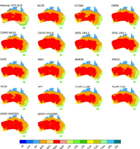
The 17 GCMs used here all give different distributions of future climate types (Fig. 2). The variability in projec-tions of climate types is consistent with the variability pre-viously reported in rainfall (Chiew et al., 2009a), runoff (Chiew et al., 2009b) and recharge (Crosbie et al., 2010b). The most variability between GCMs is seen in the tropical (A) climate types where the proportion of the continent with these climate types is projected to decrease by 8 GCMs and increase by 9 GCMs (Fig. 3), this inconsistency between GCMs across northern Australia has been reported previ-ously (CSIRO, 2009a). There is more consensus amongst the projected arid (B) climate types where 15 out of 17 GCMs

Fig. 1. Historical baseline K¨oppen-Geiger climate types for the

pe-riod 1970–2010.

project an increase in their proportion of the continent. The projections derived from all GCMs agree that the proportion of the continent covered by the temperate (C) and cold (D) climate types will decrease. The variability across GCMs in-creases as the degree of global warming inin-creases, highlight-ing the uncertainty in projecthighlight-ing future climate types, the ex-ception is for the cold (D) climate types where the proportion of the continent is approaching zero with increasing global warming.

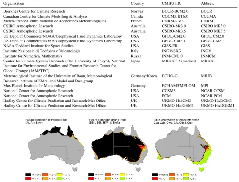
The mode of the climate types from the ensemble of GCMs was determined for each global warming scenario at the historical grid cell scale (Fig. 4) and was further simpli-fied to just the changes in top level classifications (Fig. 5). The tropical (A) climate types occur across the north of the continent and are expanding overall with increasing global warming, this is due to an expansion along the Queensland (Qld) coast (displacing temperate) that is progressing faster than the contraction inland (being replaced by arid). Over-all the tropical (A) area is projected to expand from 8.8 % of the continent under the historical baseline up to 9.1 % for +2.4◦C. The arid (B) climate types are expanding in every direction with increasing global warming; the area is pro-jected to increase from 76.5 % to 81.7 % of the continent for +2.4◦C. The greatest area of expansion is in the south-east of Queensland, but the more surprising result is that by +1.0◦_{C, the arid climate types have spread into southern}

Fig. 2. K¨oppen-Geiger climate types under a future climate of

+2.4◦C derived from 17 GCMs (historical baseline period is in-cluded for reference).

global warming to the point where there are only 2 grid cells (∼50 km2)remaining for +2.4◦C.

A summary of the changes in the proportion of the con-tinent of each climate type, at the third level of the classi-fication, are shown in Fig. 6. For Af (tropical, Rainforest), the area increases to a peak at +1.0◦_{C before declining with}

further increases in global warming to be 3 % above the his-torical baseline by +2.4◦C. The area of Am (tropical, Mon-soon) increases with increasing global warming to be 50 % above the historical baseline by +2.4◦C. The total area of the Af and Am climate types are quite small (0.04 % and 0.08 % respectively for the historical baseline), the majority of the tropical climate type is made up of Aw (tropical, Savannah; 8.7 % historical baseline). This climate type is projected to have a small increase in area with increasing global warming (8.9 % of the continent for +2.4◦C); this is caused by a con-traction in inland areas and an expansion southward along the Queensland coast.

The arid climate types cover most of the continent, of them BWh (arid, Desert, Hot) covers the most area at 39.2 % un-der the historical baseline (Fig. 6). This climate type is pro-jected to expand to the south-west, south and south-east and by +2.4◦C covers 49.4 % of the continent. Under the histor-ical baseline climate BSh (arid, Steppe, Hot) covers the sec-ond greatest area (29.2 %) and this is projected to increase to the north, east, south-east, south and south-west to a total of 31.1 % of the continent by +2.4◦C. Under the historical base-line climate BSk (arid, Steppe, Hot) had the fourth greatest area (7.4 %) but is projected to see the majority (83 %) of this

Fig. 3. Boxplots of the proportion of Australia covered by the top

level K¨oppen-Geiger climate types under a future climate derived from 17 GCMs. The grey box represents the interquartile range, the line in the box is the median, the whiskers contain 95 % of the data and the black circles are outliers. The white squares represent the mode as shown in Fig. 4. The baseline historical climate is repre-sented in this figure by a global warming of 0◦C.

Fig. 4. K¨oppen-Geiger climate types for the mode of 17 GCMs for

5 global warming scenarios (historical baseline period is included for reference).

area replaced by BSh by +2.4◦_{C. The BWk (arid, steppe,}

cold) climate type only occupies a small proportion of the continent under the historical baseline climate (0.7 %) and this is completely replaced by BWh by +2.4◦C.

The temperate (C) climate types are projected to have the greatest reduction in area under a future climate (Fig. 6). Cli-mate type Csa (temperate, dry summer, hot summer) initially decreases in area with increasing global warming to reach a minimum at +1.0◦C where it is being replaced by BSh, with further global warming Csa is displacing Csb (temper-ate, Dry Summer, Warm Summer) and by +2.4◦C occupies 1 % more area than it did under the historical baseline climate (1.1 % of the continent). Climate type Csb occupied 1.6 % of the continent under the historical baseline climate and this decreases rapidly with increasing global warming for a 70 % reduction in area by +2.4◦_{C. The Cwa (temperate, Dry}

Table 2. List of GCMs used in this study also showing the abbreviations used in Fig. 2.

Organisation Country CMIP3 I.D. Abbrev.

Bjerknes Centre for Climate Research Norway BCCR-BCM2.0 BCCR

Canadian Centre for Climate Modelling & Analysis Canada CGCM3.1(T63) CCCMA

M´et´eo-France/Centre National de Recherches M´et´eorologiques France CNRM-CM3 CNRM

CSIRO Atmospheric Research Australia CSIRO-Mk3.0 CSIRO MK3.0

CSIRO Atmospheric Research Australia CSIRO-Mk3.5 CSIRO MK3.5

US Dept. of Commerce/NOAA/Geophysical Fluid Dynamics Laboratory USA GFDL-CM2.0 GFDL CM2.0

US Dept. of Commerce/NOAA/Geophysical Fluid Dynamics Laboratory USA GFDL-CM2.1 GFDL CM2.1

NASA/Goddard Institute for Space Studies USA GISS-ER GISS

Instituto Nazionale di Geofisica e Vulcanologia Italy INGV-SXG INGV

Institute for Numerical Mathematics Russia INM-CM3.0 INMCM

Center for Climate System Research (The University of Tokyo), National Institute for Environmental Studies, and Frontier Research Center for Global Change (JAMSTEC)

Japan MIROC3.2 (medres) MIROC

Meteorological Institute of the University of Bonn, Meteorological Research Institute of KMA, and Model and Data group

Germany/Korea ECHO-G MIUB

Max Planck Institute for Meteorology Germany ECHAM5/MPI-OM MPI

National Center for Atmospheric Research USA CCSM3 NCAR CCSM

National Center for Atmospheric Research USA PCM NCAR PCM

Hadley Centre for Climate Prediction and Research/Met Office UK UKMO-HadCM3 UKMO HADCM3

Hadley Centre for Climate Prediction and Research/Met Office UK UKMO-HadGEM1 UKMO HADGEM1

Fig. 5. Future extents of the top level K¨oppen-Geiger classification – arid, tropical and temperate (cold not shown on this plot).

climate types (6.5 % of the continent). Under the future cli-mate scenarios this clicli-mate type is moving to the south-east, it is being replaced by BSh from the north-west and is replac-ing Cfb (temperate, Without Dry Season, Warm Summer) to the south-east, overall the area it occupies is projected to de-crease by 24 % by +2.4◦C. Under the future climate scenar-ios, the Cfb climate type is decreasing in area with increas-ing global warmincreas-ing, by +2.4◦C it is projected to have lost 44 % of the 4.6 % of the continent that it occupied under the historical baseline climate. The Cfc (temperate, without dry season, cold summer) climate type only occurs in small areas (0.07 % of the continent) of Tasmania (Tas) under this histor-ical baseline climate, under the future climate scenarios it is projected to be increasingly replaced by Cfb with increased global warming (94 % reduction by +2.4◦C).

The cold (D) climate types Dfb (cold, without dry sea-son, warm summer) and Dfc (cold, without dry seasea-son, cold summer) only occupy a small area (0.01 % and 0.006 %

respectively) of New South Wales and Victoria at high al-titude under the historical baseline climate. After +1.0◦C Dfc is projected to be completely replaced (by Cfb) and by +2.4◦C the projected area of Dfb is reduced by 93 %.

4 Discussion

As pointed out by Cannon (2012), at the highest level of the K¨oppen-Geiger classification it is only the arid (B) class that is discriminated by rainfall, this means that transitions in cli-mate types due to clicli-mate change may not be sensitive to changes in rainfall. For this paper, which is focused on Aus-tralia, this is not a big problem as the major transitions pro-jected in climate type involve the arid (B) climate types.

Fig. 6. The proportion of Australia covered by the K¨oppen-Geiger

climate types for 5 global warming scenarios and the mode of 17 GCMs and the change in area relative to the historical baseline sce-nario.

Fig. 7. Distribution of K¨oppen-Geiger climate types under the

present extent of annual crops and pastures (BRS, 2008) (blacked out areas of the figure do not have annual vegetation).

climate classification. In the historical baseline climate, the cold (D) climate types form a subset of the extremely high yield zone of Donohue et al. (2011) that is defined as energy limited and are responsible for a disproportionately large amount of the runoff in the Murray-Darling Basin (MDB). The change in climate type from cold (D) to temperate (C) is the result of a projected increase in temperature and there-fore potential evapotranspiration, combined with a projected decrease in rainfall (Chiew et al., 2009a) and the area that is energy limited is reduced resulting in less runoff. The area classified as cold (D) under the historical baseline climate is projected to be amongst the areas with the greatest reduction in runoff in the MDB (Chiew et al., 2009b).

The transition of areas from temperate (C) to arid (B) climate types could cause either an increase or decrease in recharge. Barron et al. (2012) showed that groundwater recharge under BSh is higher for a given annual rainfall than Cfa but BSh by definition experiences a lower rainfall than Cfa (Peel et al., 2007). The majority of the areas projected to transition from temperate (C) to arid (B) under a future cli-mate are also projected to have a reduction in recharge (Cros-bie et al., 2012), the analysis of Barron et al. (2012) suggests that the reduction in recharge would have been greater with-out the change in climate type.

Fig. 8. Comparison of the evapotranspiration and recharge for

dif-ferent vegetation derived from observed field data. The evapotran-spiration curves are derived from Fig. 9 in Zhang et al. (2001) and the recharge curves are derived from Fig. 6 in Crosbie et al. (2010a).

For a future climate of +2.4◦_{C, 24 % of the country is}

pro-jected to change climate type. This includes the disappear-ance of two climate types completely (BWk and Dfc) and five others that are projected to occupy less than one third of the area that they occupied under the historical baseline climate (BSk, Csb, Cwa, Cfc and Dfb). These changes in cli-mate type will cause changes in vegetation types that are not actively managed and potentially also a loss of biodiversity (Markham, 1996). Dynamic vegetation growth models have been used to assess the temporal (as well as spatial) scale of potential vegetation changes and in some cases it has been re-ported that vegetation change could take over 100 yr to come to equilibrium after the climate has reached a new equilib-rium (Cramer et al., 2001; Loehle, 2011). There are also ob-servations that suggest that vegetation change could occur much more rapidly, this could occur due to a catastrophic event such as forest mortality (Mitchell et al., 2012) or grad-ually over a couple of decades as has been observed through an increase in persistent vegetation (Donohue et al., 2009).

In actively managed agricultural landscapes, any change in vegetation type will result from socio-economic factors rather than climate change alone (Holman, 2006). This will occur when it is no longer profitable to grow crops. Under the historical baseline climate only the northern wheatbelt (WA) has a significant area of annual vegetation in the BSh climate type (Fig. 7). The northern wheatbelt is currently amongst the lowest yielding grain growing areas in the country (Kokic et al., 2005). The majority of annual cropping is undertaken in temperate (C) or BSk climate types, and under the cur-rent distribution of cropping zones there is nowhere in Aus-tralia where there is annual vegetation under the BWh cli-mate type. Under a +2.4◦_{C future climate BWh has moved}

climate types (Farre and Foster, 2010; Wang et al., 2009; Luo et al., 2005).

If areas that are currently under annual crops and pastures change to another land use due to climate change, then there will be a corresponding hydrological impact. For example, the northern wheatbelt (WA) is projected to have a 10–20 % reduction in recharge for a median 2050 climate assuming that the vegetation type remains static (Crosbie et al., 2012). However, if the vegetation were to revert to a more natu-ralised state of perennial vegetation then the recharge could be reduced by at least double the amount projected for cli-mate change directly (Fig. 8). In this example the direct and indirect effects of climate change upon groundwater recharge are compounded (i.e. a positive feedback).

The largest transition in climate types projected for +2.4◦_{C is from temperate (C) to arid (B); this could cause}

a transition in vegetation type in some areas from forest to grassland. Many of the forested areas of south-east Australia are projected to have a decrease in runoff due to reduced rain-fall under a future climate (Chiew et al., 2009b). Some of these areas are also projected to have a change in climate type from temperate (C) to arid (B). Zhang et al. (2001) showed that for a given annual rainfall, forests have greater evap-otranspiration than grassland and consequently less runoff (Fig. 8). If reduced rainfall under a future climate results in a transition from forest to grassland, then the effects of re-duced rainfall upon runoff could be mitigated by a reduction in evapotranspiration from the vegetation change (i.e. a neg-ative feedback).

5 Conclusions

This paper has presented projections of K¨oppen-Geiger cli-mate types across Australia for future clicli-mates based upon 17 GCMs and five global warming scenarios. There is no con-sensus amongst the GCMs in the projections for the Tropics (A), where nine GCMs project an increase in area and eight project a decrease. The mode of the GCMs shows an increase of 0.3 % in area for a global warming scenario of +2.4◦C to 9.1 % from 8.8 % under the historical baseline climate. For the arid (B) climate types 15 out of 17 GCMs project an in-crease in area with a mode of 81.7 % of the continent for +2.4◦C compared to 76.5 % under the historical baseline cli-mate. All 17 GCMs project reductions in the temperate (C) and cold (D) climate types. The increase in the area covered by the arid (B) climate types is balanced by a reduction in the temperate (C) climate types with the historical baseline climate being 14.7 % of the continent and this is projected to reduce to 9.2% for a +2.4◦C future climate. The cold (D) climate types only occupy a very small part of the continent under the historical baseline climate (0.016 %) and this is re-duced by 95 % under a +2.4◦C future climate.

Under a warmer drier climate, previous studies have made projections for reductions in runoff and recharge over large

parts of Australia assuming static vegetation coverage. As the K¨oppen-Geiger climate classification was developed based upon the distribution of vegetation it may provide a useful surrogate for vegetation change projections under a future climate. If vegetation change were to be incorporated into fu-ture projections of water resources availability it could pro-vide different results. A transition in vegetation type from annual cropping to perennial grassland would have a com-pounding effect on a reduction in recharge, whereas a transi-tion from forest vegetatransi-tion to grassland would have a mitigat-ing effect upon a reduction in runoff. Therefore, it is recom-mended that detailed research is necessary to incorporate the indirect effects of climate change due to vegetation change into studies of climate change impacts upon water resources in Australia.

Acknowledgements. The authors would like to acknowledge the

National Water Commission for providing funding to support the

Climate Change Impacts on Groundwater Resources project under

the National Groundwater Action Plan and CMIP3 for providing GCM outputs.

Edited by: Y. Fan

References

Barron, O. V., Crosbie, R. S., Pollock, D., Dawes, W. R., Charles, S. P., Pickett, T., and Donn, M.: Climatic controls on diffuse groundwater recharge across Australia, Hydrol. Earth Syst. Sci. Discuss., 9, 6023–6062, doi:10.5194/hessd-9-6023-2012, 2012. BRS: Integrated Vegetation Cover 2008, Bureau of Rural Sciences,

Canberra, 2008.

Budyko, M. I.: Climate and Life, International Geophysics, Aca-demic Press, 508 pp., 1974.

Cannon, A. J.: K¨oppen versus the computer: comparing K¨oppen-Geiger and multivariate regression tree climate classifications in terms of climate homogeneity, Hydrol. Earth Syst. Sci., 16, 217– 229, doi:10.5194/hess-16-217-2012, 2012.

Chiew, F. H. S., Teng, J., Vaze, J., and Kirono, D. G. C.: Influence of global climate model selection on runoff impact assessment, J. Hydrol., 379, 172–180, 2009a.

Chiew, F. H. S., Teng, J., Vaze, J., Post, D. A., Perraud, J. M., Kirono, D. G. C., and Viney, N. R.: Estimating climate change impact on runoff across southeast Australia: Method, results, and implications of the modeling method, Water Resour. Res., 45, W10414, doi:10.1029/2008WR007338, 2009b.

Cramer, W., Bondeau, A., Woodward, F. I., Prentice, I. C., Betts, R. A., Brovkin, V., Cox, P. M., Fisher, V., Foley, J. A., Friend, A. D., Kucharik, C., Lomas, M. R., Ramankutty, N., Sitch, S., Smith, B., White, A., and Young-Molling, C.: Global re-sponse of terrestrial ecosystem structure and function to CO2

and climate change: results from six dynamic global vegetation models, Glob. Change Biol., 7, 357–373, doi:10.1046/j.1365-2486.2001.00383.x, 2001.

predict recharge in data-poor areas?, Hydrol. Earth Syst. Sci., 14, 2023–2038, doi:10.5194/hess-14-2023-2010, 2010a.

Crosbie, R. S., McCallum, J. L., Walker, G. R., and Chiew, F. H. S.: Modelling the climate change impact on groundwater recharge in the Murray-Darling Basin, Hydrogeol. J., 18, 1639–1656, 2010b. Crosbie, R. S., Pickett, T., Mpelasoka, F. S., Hodgson, G., Charles, S. P., and Barron, O. V.: An assessment of the climate change impacts on groundwater recharge at a continental scale using a probabilistic approach with an ensemble of GCMs, Climatic Change, online first: doi:10.1007/s10584-012-0558-6, 2012. CSIRO: Water availability in the Murray-Darling Basin. A report

to the Australian Government from the CSIRO Murray-Darling Basin Sustainable Yields Project, CSIRO: Water for a Healthy Country National Research Flagship, Australia, 67 pp., 2008. CSIRO: Water in northern Australia: Summary of reports to the

Australian Government from the CSIRO Northern Australia Sus-tainable Yields Project, CSIRO: Water for a Healthy Country Na-tional Research Flagship, Canberra, 2009a.

CSIRO: Water yields and demands in south-west Western Australia: Summary of a report to the Australian Government from the CSIRO SWSY Project, CSIRO: Water for a Healthy Country Na-tional Research Flagship, 2009b.

CSIRO: Water availability for Tasmania: CSIRO Tasmania Sustain-able Yields Project, CSIRO: Water for a Healthy Country Na-tional Research Flagship, Canberra, 2009c.

Donohue, R. J., McVicar, T. R., and Roderick, M. L.: Climate-related trends in Australian vegetation cover as inferred from satellite observations, 1981–2006, Glob. Change Biol., 15, 1025– 1039, 2009.

Donohue, R. J., Roderick, M. L., and McVicar, T. R.: Assess-ing the differences in sensitivities of runoff to changes in cli-matic conditions across a large basin, J. Hydrol., 406, 234–244, doi:10.1016/j.jhydrol.2011.07.003, 2011.

Farre, I. and Foster, I.: Impact of climate change on wheat yields in Western Australia. Will wheat production be more risky in the fu-ture?, Food Security from Sustainable Agriculture, Proceedings of 15th Agronomy Conference, Lincoln, New Zealand, 2010. Fowler, H. J., Blenkinsop, S., and Tebaldi, C.: Linking climate

change modelling to impacts studies: recent advances in down-scaling techniques for hydrological modelling, Int. J. Climatol., 27, 1547–1578, doi:10.1002/joc.1556, 2007.

Holman, I. P.: Climate change impacts on groundwater recharge: uncertainty, shortcomings and the way forward?, Hydrogeol. J., 14, 637–647, 2006.

Holman, I. P., Allen, D. M., Cuthbert, M. O., and Goderniaux, P.: Towards best practice for assessing the impacts of climate change on groundwater, Hydrogeol. J., 20, 1–4, doi:10.1007/s10040-011-0805-3, 2012.

IPCC: Climate Change 2007: The Physical Science Basis. Contri-bution of Working Group 1 to the Fourth Assessment Report of the Intergovernmental Panel on Climate Change, edited by: Solomon, S., Qin, D., Manning, M., Chen, Z., Marquis, M., Av-eryt, K. B., Tignor, M., and Miller, H. L., Cambridge University Press, Cambridge UK, 996 pp., 2007.

Jones, D. A., Wang, W., and Fawcett, R.: High-quality spatial climate data-sets for Australia, Australian Meteorological and Oceanographic Journal, 58, 233–248, 2009.

Kleidon, A., Fraedrich, K., and Heimann, M.: A Green Planet Ver-sus a Desert World: Estimating the Maximum Effect of

Vegeta-tion on the Land Surface Climate, Climatic Change, 44, 471–493, doi:10.1023/a:1005559518889, 2000.

Kokic, P., Heaney, A., Pechey, L., Crimp, S., and Fisher, B. S.: Cli-mate change, predicting the impacts on agriculture: a case study, Australian Commodities, 12, 161–170, 2005.

K¨oppen, W.: Das geographisca System der Klimate, in: Handbuch der Klimatologie, edited by: K¨oppen, W. and Geiger, G., Born-traeger, 1–44, 1936.

K¨oppen, W.: Die W¨armezonen der Erde, nach der Dauer der heis-sen, gem¨assigten und kalten Zeit und nach der Wirkung der W¨arme auf die organische Welt betrachtet (The thermal zones of the earth according to the duration of hot, moderate and cold periods and to the impact of heat on the organic world), Mete-orol. Z., 1, 215–226, 1884, translated and edited by: Volken, E. and Br¨onnimann, S., Meteorol. Z., 220, 2351–2360, 2011. Kottek, M., Grieser, J., Beck, C., Rudolf, B., and Rubel, F.: World

map of the K¨oppen-Geiger climate classification updated, Mete-orol. Z., 15, 259–263, 2006.

Loehle, C.: Criteria for assessing climate change impacts on ecosys-tems, Ecology and Evolution, 1, 63–72, 2011.

Luo, Q., Bellotti, W., Williams, M., and Bryan, B.: Potential impact of climate change on wheat yield in South Australia, Agr. Forest Meteorol., 132, 273–285, 2005.

Markham, A.: Potential impacts of climate change on ecosystems: A review of implications for policymakers and conservation bi-ologists, Clim. Res., 6, 179–191, doi:10.3354/cr006179, 1996. Meehl, G. A., Covey, C., Delworth, T., Latif, M., McAvaney,

B., Mitchell, J. F. B., Stouffer, R. J., and Taylor, K. E.: The WCRP CMIP3 multimodel dataset – A new era in cli-mate change research, B. Am. Meteorol. Soc., 88, 1383–1394, doi:10.1175/BAMS-88-9-1383, 2007.

Mitchell, P. J. M., O’Grady, A. P., and Pinkard, E. A.: Defining past and future climate drivers of drought induced tree mortality: a case study from southern Australia, in preparation, 2012. Mitchell, T. D.: Pattern scaling – An examination of the accuracy

of the technique for describing future climates, Climatic Change, 60, 217–242, doi:10.1023/a:1026035305597, 2003.

Mpelasoka, F. S. and Chiew, F. H. S.: Influence of Rainfall Scenario Construction Methods on Runoff Projections, J. Hydrometeorol., 10, 1168–1183, 2009.

Nakicenovic, N. and Swart, R.: Special Report on Emission Scenar-ios, Intergovernmental Panel on Climate Change, 612 pp., 2000. Peel, M. C., Finlayson, B. L., and McMahon, T. A.: Updated world map of the K¨oppen-Geiger climate classification, Hy-drol. Earth Syst. Sci., 11, 1633–1644, doi:10.5194/hess-11-1633-2007, 2007.

Post, D. A., Chiew, F. H. S., Teng, J., Viney, N. R., Ling, F. L. N., Harrington, G., Crosbie, R. S., Graham, B., Marvanek, S., and McLoughlin, R.: A robust methodology for conducting large-scale assessments of current and future water availability and use: A case study in Tasmania, Australia, J. Hydrol., 412–413, 233–245, doi:10.1016/j.jhydrol.2011.02.011, 2012.

Prentice, I. C., Cramer, W., Harrison, S. P., Leemans, R., Monserud, R. A., and Solomon, A. M.: A Global Biome Model Based on Plant Physiology and Dominance, Soil Properties and Climate, J Biogeogr., 19, 117–134, 1992.

doi:10.1127/0941-2948/2010/0430, 2010.

Rubel, F. and Kottek, M.: Comments on: The thermal zones of the Earth by Wladimir Koppen (1884), Meteorol. Z., 20, 361–365, 2011.

Suppiah, R., Hennessy, K., Whetton, P. H., McInnes, K., Macadam, I., Bathols, J., Ricketts, J., and Page, C. M.: Australian climate change projections derived from simulations performed for the IPCC 4th Assessment Report, Aust. Meteorol. Mag., 56, 131– 152, 2007.

Wang, E., Cresswell, H., Bryan, B., Glover, M., and King, D.: Mod-elling farming systems performance at catchment and regional scales to support natural resource management, NJAS-Wagen. J. Life Sc., 57, 101–108, 2009.