ScholarWorks @ Georgia State University
Economics Dissertations Department of Economics
Fall 12-15-2010
Three Essays on the Search for Economic Efficiency
Jason J. DelaneyGeorgia State University
Follow this and additional works at:https://scholarworks.gsu.edu/econ_diss
Part of theEconomics Commons
This Dissertation is brought to you for free and open access by the Department of Economics at ScholarWorks @ Georgia State University. It has been accepted for inclusion in Economics Dissertations by an authorized administrator of ScholarWorks @ Georgia State University. For more information, please [email protected].
Recommended Citation
PERMISSION TO BORROW
In presenting this dissertation as a partial fulfillment of the requirements for an advanced degree from Georgia State University, I agree that the Library of the University shall make it available for inspection and circulation in accordance with its regulations governing materials of this type.
I agree that permission to quote from, to copy from, or to publish this dissertation may be granted by the author or, in his or her absence, the professor under whose direction it was written or, in his or her absence, by the Dean of the Andrew Young School of Policy Studies. Such quoting, copying, or publishing must be solely for scholarly purposes and must not involve potential financial gain. It is understood that any copying from or publication of this dissertation which involves potential gain will not be allowed without written permission of the author.
NOTICE TO BORROWERS
All dissertations deposited in the Georgia State University Library must be used only in accordance with the stipulations prescribed by the author in the preceding statement.
The author of this dissertation is:
Jason J. Delaney 1686 Glencove Ave SE Atlanta, GA 30317
The director of this dissertation is:
James C. Cox
Experimental Economics Center
Andrew Young School of Policy Studies Georgia State University
14 Marietta Street, NW Atlanta, GA 30303
Users of this dissertation not regularly enrolled as students at Georgia State University are required to attest acceptance of the preceding stipulations by signing below. Libraries borrowing this dissertation for the use of their patrons are required to see that each user records here the information requested.
Type of use
THREE ESSAYS ON THE SEARCH FOR ECONOMIC EFFICIENCY
By
JASON JAMES DELANEY
A Dissertation Submitted in Partial Fulfillment of the Requirements for the Degree
of
Doctor of Philosophy in the
Andrew Young School of Policy Studies of
Georgia State University
Copyright by Jason James Delaney
ACCEPTANCE
This dissertation was prepared under the direction of the candidate’s Dissertation Committee. It has been approved and accepted by all members of that committee, and it has been accepted in partial fulfillment of the requirements for the degree of Doctor of Philosophy in Economics in the Andrew Young School of Policy Studies of Georgia State University.
Dissertation Chair: James C. Cox
Committee: Jane G. Gravelle
Jorge Martinez-Vazquez Vjollca Sadiraj
Electronic Version Approved:
Mary Beth Walker, Dean
Andrew Young School of Policy Studies Georgia State University
iv
ACKNOWLEDGMENTS
As I completed the following dissertation, I had the unique and irreproducible
pleasure of working with some of my favorite people; my only regret is that the solitary
work of a graduate student did not afford me more opportunities to work more closely
with them. It is my hope that the luxurious existence of the tenure-track assistant
professor will give me some opportunities to work with them again—if not then, well,
there’s always tenure.
First, I wish to thank Jim Cox. His example, as a scholar, a scientist, and an ardent
pursuer of truth, is one I hope to follow. His passion for the field deserves credit for
bringing me into the experimental fold, and his advice and encouragement have improved
the nascent ideas with which he was presented and pushed me to become a better and
more rigorous researcher. There’s no place quite like the lab, and I owe Jim a debt of
gratitude for getting me in there.
The second paper would never have been written if not for Jane Gravelle’s
insistence that I do the thing right. She pushed me to concern myself not with the feasible
but with the ideal, and then find a way to make it happen—and that lesson will improve
all the work I ever do. Jorge Martinez-Vazquez pushed me to improve the dissertation as
a whole, and the second essay in particular. His policy focus and his expertise are an
inspiration, and his sense of humor is one I always find refreshing.
Vjollca Sadiraj made the third paper possible. Her intellectual rigor and curiosity,
her willingness to entertain almost any idea for the sake of argument, and her shared
inability to let a good discussion die—all of these make her one of my favorite
v
I would be remiss if I did not extend gratitude also to those who have helped me
through this process. Todd Swarthout and Kevin Ackaramongkolrotn have been essential
in my development as an experimentalist. Sarah Jacobson has been a peerless
collaborator, and William Holmes and Daniel Hall, my co-sufferers through the
wonderful, terrible dissertation process. Thank you also to the participants in the
workshops and seminars upon whom I have inflicted less than finished versions of the
essays within. Financial support for the research in Chapter I came from Georgia State
University.
Finally, there is the way one envisions completing a dissertation, and the way it
actually happens. Thank you to my wife, Cheryl, for helping to make it actually happen.
Thank you to my daughter, Violet, who slept as an infant in my arms when I came up
vi CONTENTS
TABLES ... viii
FIGURES ... ix
ABSTRACT ... x
Chapter I: An Experimental Test of the Pigovian Hypothesis ... 1
Introduction ... 1
Theory ... 5
Protocol ... 9
Hypotheses ... 14
Results ... 16
Conclusion ... 26
Chapter II: Apples to Apples to Oranges ... 29
Introduction ... 29
Cost and Comparability in States and Cities... 35
Several Methods... 39
What Determines Public Expenditures? ... 44
Comparing Apples to Apples to Oranges ... 48
Conclusion ... 60
Chapter III: Evading Nash Traps in Two-Player Simultaneous Games: ... 62
Introduction ... 62
Theory of Mind, the Categorical Imperative, and Agents ... 66
Modeling agents ... 69
Properties of strategic concepts ... 70
Détente and No-Initiative Strategic Concepts... 72
Détente and No-Initiative in Two-Player Games... 77
Conflict games ... 77
Social dilemmas ... 78
Constant-sum games ... 80
vii
Appendix A. Subject Instructions for the Pigovian Subsidy Experiment ... 83
Appendix B. Tutorial Screenshots ... 91
Appendix C. Estimates of Per-Capita Expenditure Need by State ... 100
Appendix D. Estimates of Per-Capita Expenditure Need by Sub-State Area ... 102
Appendix E. Workload and Expenditure Need Calculations Under the ACIR Approach ... 114
Appendix F: Proofs of Results in ―Evading Nash Traps in Two-Player Simultaneous Games‖ ... 117
viii
LIST OF TABLES
Table Page
1. Statistical tests of hypotheses and robustness checks ... 17
2. Tests of the effect of the Decrease treatment ... 22
3. Regression results under different specifications ... 24
4. Seven approaches to estimating fiscal need in the United States ... 41
5. Regression results from pooled MSA-level SUR ... 49
6. Top 5, Median, and Bottom 5 States and sub-state areas by fiscal need ... 51
7. Correlation coefficients for different measures of expenditure need ... 52
8. The difference in regression-based expenditure need estimates dependent on land area and population density ... 57
ix
LIST OF FIGURES
Figure Page
1. Information treatment ... 12
2. Tutorial screenshot ... 13
3. Payoff calculator ... 14
4. Mean BLUE investment by period by session ... 18
5. Investment decisions by period, Subsidy Session... 18
6. Investment decisions by period, Information Session ... 20
7. Absolute deviation from best-response by period by session ... 26
8. Per-capita state-and-local direct expenditure by state in 2002 ($1,000) ... 35
9. Measures of state expenditure need by state population density ... 38
10. Kernel density estimates of hybrid, state-based, and traditional RES estimates against actual expenditures... 54
11. Measures of sub-state-level expenditure need by sub-state population density ... 55
12. Hybrid-regression RES results across States ... 56
13. State-based regression vs. Hybrid-regression ... 56
14. Traditional estimates of fiscal need vs. Hybrid estimates ... 58
15. Hybrid estimate of fiscal need vs. Actual per-capita expenditure ... 59
16. Four-stage centipede game ... 64
17. Traveler’s Dilemma ... 64
18. Nash equilibrium, détente strategic, and no-initiative strategic profiles in a two-player game ... 74
19. Purely ordinal conflict games with different NE and NIS profiles ... 77
20. The Prisoner’s Dilemma and an abbreviated Traveler’s Dilemma ... 79
x ABSTRACT
ESSAYS ON THE SEARCH FOR ECONOMIC EFFICIENCY
By
Jason James Delaney
July 2010
Committee Chair: Dr. James C. Cox
Major Department: Economics
The chapters of this dissertation examine efficiency failures in three areas of
applied microeconomics: experimental economics, public finance, and game theory. In
each case, we look at ways to resolve these failures to promote the public good.
The first chapter, ―An Experimental Test of the Pigovian Hypothesis,‖ looks at
two different policies designed to reduce congestion in a common-pool resource (CPR).
The predictive power of game-theoretic results with respect to an optimal subsidy in a
common-pool resource game remains an open question. We present an experiment with
training and a simplified decision task, allowing more tractable computerized CPR
experiments. We find that subject behavior converges to the Nash prediction over a
number of periods. A Pigovian subsidy effectively moves subject behavior to the
pre-subsidy social optimum. Finally, we find a significant but non-persistent effect of
information provision in moving subjects toward the social optimum.
The second chapter, ―Apples to Apples to Oranges,‖ looks at efficiency and
equity failures across states resulting from public expenditure. The literature on fiscal
equalization and horizontal equity has established that measures of fiscal capacity should
xi
provide services given an average level of revenue. This chapter introduces an extension
of the Representative Expenditure System that uses regression methods and both state
and metropolitan statistical area (MSA) level data, allowing for comparability of input
costs, service requirements, and levels of need. The regression-based results are robust
across state- and MSA-level formulations, although state-level approaches overestimate
need for larger, less populous states. All regression-based results diverge from previous
workload-based approaches.
The third chapter, ―Evading Nash Traps in Two-Player Simultaneous Games,‖
looks at efficiency failures in two-player simultaneous games. In some important games,
Nash equilibrium selects Pareto-inferior equilibrium profiles. Empirically, Nash
equilibrium sometimes performs poorly when predicting actual behavior. Previous
approaches rely on repetition or external correlation to support efficient outcomes in
simultaneous games. This chapter presents two new concepts: ―détente‖ and
―no-initiative,‖ in which players consider their own strategies and other-best-responses. We
Chapter I: An Experimental Test of the Pigovian Hypothesis
Introduction
Many of the most important policy questions of our time relate not to privately
consumed goods, but to the unintended consequences of consumption of goods, broadly
referred to as externalities. Carbon emissions, obesity, and the stability of financial
firms—they all have consequences that extend beyond those involved in making the
economic decisions. A classic model to describe externalities is that of the common-pool
resource (CPR), and a classic solution to the problem of externalities is a Pigovian tax or
subsidy. The theoretical implications of consumption of a CPR by self-interested agents
are straightforward, but the robustness of those results is less clear. This paper addresses
several related issues: first, the literature has presented mixed results with respect to the
performance of the self-interested Nash equilibrium in predicting subject behavior.
Second, this paper presents an experimental test of the use of a Pigovian subsidy to
induce socially optimal behavior. Finally, we ask whether, given the economic and
political costs of introducing such a policy, there are other, nonmonetary ways to induce
socially preferred behavior.
This paper introduces a laboratory limited-access CPR experiment designed to
test the theory and examine potential policies to achieve improvements in governing
common-pool resources. Our experiment offers important contributions to: the public
finance literature by testing the theory of Pigovian taxation; the social preferences
literature by presenting data on the comparative results of two different policy tools—
2
that it presents a simple design making common-pool resources more tractable for future
experimental analysis.
In general, the literature has had a mixed response with respect to an important
question: does self-interested Nash equilibrium predict subject behavior toward an open-
or limited-access CPR? In their baseline experiment, Ostrom et al. (1994) (OGW) find
that subjects appropriate from a CPR at a suboptimal level—there is congestion—but that
subjects’ observed choices do not achieve a stable equilibrium. Walker et al. (1990) find
that the subjects over-consume by more than the Nash prediction, while Budescu et al.
(1995) also find that subjects over-consume, but by less than the Nash prediction. Bru et
al. (2003) find that even strategically irrelevant factors affect behavior. Rodriguez-Sickert
et al. (2008) present a CPR game with fines and find that even low fines have high
deterrence power, and that a fine which is voted down nonetheless establishes a norm.
Velez et al. (2009) find that subjects balance self-interest with conformity when selecting
strategies. Cox et al. (2009) find that first movers’ choices in a common property version
of the investment game are more likely to increase the size of the pie—and efficiency—
than in the private property version; neither version accords with the Nash prediction.
This lack of consensus in the previous literature is perhaps unsurprising. In
environments with pure private goods and institutions of impersonal exchange, Nash
equilibrium under the assumption of self-interested agents does an excellent—but not
perfect—job of predicting behavior. This is in contrast to the line of research concerning
pure public goods, following, among others, Isaac and Walker (1988), and Marwell and
Ames (1979). The deviations from the self-interested Nash equilibrium have been so
has led to the flourishing of the other-regarding preferences literature (Isaac and Walker
2003).
Perhaps theory and behavior diverge due to other-regarding preferences. The
effects of these preferences on both predicted behavior and optimal policy depend greatly
upon how the utility or consumption of others is incorporated into one’s own preferences.
In the cases of pure and impure (or ―warm-glow‖) altruism, for example, the optimal
Pigovian tax will be the same as in the self-regarding case, but the level of consumption
of the CPR will differ from the Nash prediction. Paternalistic altruism, however, implies
a higher optimal tax than the one under self-interest, because the social optimum requires
less consumption than under the presumption of self-interest (Johansson 1997)1.
Another reason equilibrium predictions might fail could be the difficulties present
in modeling the situation experimentally. In practice, creating congestion in an
experimental setting presents a formidable task, particularly in a framework that allows
simple testing of a Pigovian subsidy. This problem derives from the fact that congestion
requires a nonlinearity in payoffs such that total social payoff peaks and declines at an
overcongested—and privately optimal—level of consumption. This has the side effect of
reducing the incentive to think very hard about it at the margin, because the marginal
return to social payoff is closest to zero at the social optimum and the marginal private
return is closest to zero at the overcongested level of consumption. Because of the payoff
structure, determining the optimal strategy can be difficult, which may cause Nash
1 Briefly, the intuition for pure altruism derives from the assumption that the utility from own-consumption
4
predictions to perform poorly. If subjects are confused or frustrated, they may simply
(and rationally) decide not to think too hard about it. In one treatment, OGW allow (and
record) communication, and note that in some of their experiments, this lack of
dominance appears to be a problem. When CPR consumption increased in one period, the
group members tried to determine whether greed or error was to blame, and one member
noted that a defector would have earned ―Just a few darn cents above the rest of us.‖
The predictive power of Nash equilibria with respect to CPR games directly
affects the theoretical efficacy of Pigovian taxation or subsidies as a means to achieving
efficiency. One of the earliest and simplest solutions to congestion under an open- or
limited-access property regime, the Pigovian hypothesis has, to our knowledge, never
been tested experimentally. Pigou (1920) hypothesized that, to offset congestion, an
optimal tax or subsidy could be applied to internalize the congestion externality—
essentially altering the game so that the socially optimal outcome of the CPR is the Nash
equilibrium outcome of the modified system. If the Nash equilibrium strategy profile fails
to predict behavior in a CPR game, it is unclear what to expect from a Pigovian subsidy.
Finally, the costs of monitoring and enforcement—be they technical or political—
required to implement and maintain a Pigovian scheme are often prohibitive. To the
extent that people are motivated by non-monetary factors—other-regarding preferences,
conformity and other social norms, or merely cognitive difficulty—it may be possible to
reduce deadweight welfare loss through non-monetary means.
In order to try to minimize dominance effects, the present experiment reduces the
complexity of the payoff function, provides an intuitive interface and response mode, and
cognitive costs of decision-making to allow a sharper test of the Nash equilibrium
prediction in this CPR game. This experiment provides evidence that subjects’ choices
converge, but that it takes some time to reach the predicted outcome.
To date, there has been incidental evidence with respect to the performance of a
Pigovian subsidy in achieving the intended outcome, but there has been no direct test of
the theory. This experiment presents an experimental test of the Pigovian hypothesis; the
experimental results fit well with the theoretical prediction—Pigou was correct. A second
treatment in this paper presents subjects with information on the social optimum as a test
for the effect of such information on subjects’ behavior. We find a small and
non-persistent effect, but further experimental study is warranted to determine the feasibility
of information provision as a means of improving efficiency.
The paper is set up as follows: The next section presents the basic model of a
limited-access CPR that we use in this experiment. Section 2 presents the experimental
design, the hypotheses, and the statistical approach. Section 3 presents the results and a
discussion and Section 4 presents some concluding comments.
Theory
The theory of limited-access common-pool resources is a standard in public
finance, and environmental, urban and regional economics. The intuition derives from a
difference between the marginal private benefit (MPB) or cost (MPC) from consumption,
and the marginal social benefit (MSB) or cost (MSC) of consumption—an externality.
Assuming MPB > MSB and MPC = MSC, for example, the marginal social cost at
6
quantity will be less than the equilibrium quantity. Pigou asserted that there exists a
subsidy (or tax), t*, that will induce the socially optimal quantity choice, and that t* is
simply the difference between the net MSB and net MPB at the optimal quantity.
The theory itself is relatively straightforward, but the design of an experimental
framework to represent congestion has proven complicated. In general, CPR games,
including OGW, represent the CPR using a production function approach with an
―outside option,‖ which is a pure private good. A test of the Pigovian hypothesis can be
implemented by increasing the opportunity cost of expenditure on the CPR, by increasing
the private return to the outside option. In order to avoid potential subjective
considerations surrounding subjects’ concept of taxation, as well as to avoid negative
returns and potential effects due to prospective losses, we test the theory using a subsidy,
rather than a tax.
Formally, let index individual agents. Let represent individual i's
endowment, , represent i's expenditure on the CPR, and represent total (combined)
expenditure on CPR (including i). Let represent the payoff from an outside
option, , the payoff from the CPR, and an individual’s total payoff.
Specify the payoff to the common pool resource by defining
where β is a per-token payoff to the CPR that declines with increasing consumption of
the CPR with the γ parameter (for γ = 0, there is no congestion). Under standard
economic assumptions, each individual is maximizing with respect to . In
incentive to consume the outside option. The game played in the present experiment has
the following payoff function2:
To help subjects determine their payoffs, the software provides a payoff calculator
that allows subjects to examine hypothetical situations before making a decision. The
calculator is discussed further in section 2.
This payoff function presents subjects with a fixed per-token return to the outside
option and a declining per-token return to the CPR. In order to introduce a subsidy, we
add an additional fixed per-token amount to the return to the outside option.
Proposition. Define the payoff function for individual i as:
Without a subsidy , the Nash equilibrium is symmetrical with each
player choosing
.
For , the social optimum occurs when each player chooses
.
The socially optimal level of consumption and the Nash equilibrium level of consumption
are only identical for n = 1 or β = α.3
For , the strategy at the Nash equilibrium becomes
, and the
optimal Pigovian subsidy is
. 4
2
This is similar, but not identical, to the payoff function used in OGW (although the solutions are the same). In particular, OGW use an approach where each subject earns a share of quasi-linear production in the CPR, in which the framing and the functional form are presented to the subjects. We use a per-token approach, explained as such, which seems more transparent, and requires no facility with exponents to figure out one’s own payoff.
3 These represent two trivial cases: the case of individual use, in which there is no externality, and the case
8
The incentives governing the marginal decision to consume the CPR warrant a
brief discussion. Unlike linear VCM games, the marginal per-capita return (MPCR) is not
constant in this game. Consider a unit increase in the consumption of the CPR (implying
a unit decrease in consumption of the outside option), and where represents the current
level of CPR consumption. The MPCR to oneself (which is the previously discussed
MPB) from consuming an additional unit of the CPR is –
– . The MPCR to others varies across individuals, proportional with their level of
consumption of the CPR, and is equal to – for each individual, where indexes other
individuals. This is straightforward: each unit of CPR consumption carries a variable
benefit, which is for the th unit, carries an opportunity cost in the
form of a forgone return to the outside option, , and reduces the value of all
previous consumption of the CPR by , which decreases own-payoff by (fishing or
driving congests own-consumption as well), and decreases other payoffs by for each
k in the group. Except for the case where no one else is currently consuming the CPR,
one’s own consumption of the CPR unambiguously reduces others’ payoffs: MSB <
MPB for .
4 For the purposes of this experiment, we are abstracting away from the source of the subsidy and possible
Protocol
Because the impact of social norms and framing seems non-trivial, we avoid
terminology like ―common-pool resource,‖ ―extraction,‖ ―appropriation,‖ ―tax,‖
―subsidy,‖ etc. We follow Andreoni and Petrie (2004) in presenting the decision they face
as an ―investment‖ decision in which they will decide how to invest a number of tokens
in each period. Subjects are given the choice to invest their tokens in the outside option or
the CPR, which are referred to in the experiment as the ―RED investment‖ and the
―BLUE investment,‖ respectively.
We implement this model using the following parameterization: (α: per-token
baseline RED payoff; β: per-token starting BLUE payoff; γ: per-token BLUE congestion
parameter; δ: per-token RED subsidy; z: period endowment; n: group size) = ($0.00,
$0.36, $0.01, $0.12, 10, 3). These parameters were chosen for a number of reasons. In
particular, they guarantee a unique (and symmetric) interior Nash equilibrium in both the
baseline and the subsidy treatments ( and , respectively). They also provide
enough distance between the two equilibria for statistical inference. In addition, the
differences are economically significant. Under the socially optimal outcome, subjects
would earn $26.88; the per-subject payment under the Nash equilibrium outcome is
$22.26. The minimum possible payoff is $0.00 for the information treatment and $4.20
for the subsidy treatment. The maximum possible payoff is $54.60 under both conditions.
Finally, the group size is such that off-Nash behavior might reasonably be sustained, as
implicit collusion is easier with smaller groups. If Nash cannot be rejected, it seems likely
10
This analysis has relied on continuity and differentiability to determine Nash
results. In practice, it is not generally true that a unique Nash equilibrium in the
continuous case implies a unique equilibrium in a discrete implementation (Swarthout
and Walker 2009). In order to ensure that these continuous results hold for the
implementation we use in the experiment, we tested every strategy profile under the
parameters and find that there is indeed a unique (and symmetric) interior Nash
equilibrium in both the baseline case and the subsidy case
.
The experiment was conducted in two sessions at Georgia State University’s
Experimental Economics Center (ExCEN). In each session there were 24 subjects,
randomly separated into 8 groups of 3.5 Each session lasted about an hour and a half.
Individual earnings, including a $5 show-up payment, ranged from $17.98 to $40.60.
The sessions were run with a double-blind protocol. Our primary research
questions concern individual behavior under induced preferences, as well as those
preferences they might have regarding the welfare of anonymous members of their group.
In addition, the information treatment looks at information provision without a direct
appeal to social norms. There is some experimental evidence that with less than strict
anonymity, the domain of other-regarding preferences may expand beyond the group
(see, for example, Hoffman et al. (1994), Cox and Deck (2006), and Andreoni and Petrie
(2004)). Relaxing anonymity to observe CPR consumption decisions in the presence of
external subjective norms is another straightforward extension of the present experiment.
5
Strict anonymity was maintained, but in each round, all subjects were aware of
the sum of the decisions made by the other members of their group in each previous
round. Groups were randomly assigned, but fixed throughout the experiment. The
experiment was computerized, and was run in an experimental lab with dividers in place
so that subjects could not easily see one another. Each subject participated in two
baseline treatments and one of two experimental treatments: either the Pigovian subsidy
treatment or the information treatment. All subjects in a given session participated in the
same treatments. For each treatment, each individual was asked to make seven
―investment‖ decisions.
In each period, each token invested in the RED investment paid a fixed per-token
amount. Each token invested in the BLUE investment paid a per-token amount that
depended upon the total number of tokens invested in the BLUE investment by the group.
Each session consisted of two treatments, administered in B-A-B format, so that each
session consisted of a baseline treatment, an experimental treatment, and a second
baseline treatment. Subjects knew the number of periods, but were not made aware ahead
of time when treatments would begin or end. Because of the relative complexity of the
payoff structure as well as an established downward trend, or ―decay,‖ in group
contributions, widely documented in public goods games (Isaac and Walker 1988, for
example), providing a second baseline allows us to observe, and perhaps account for, any
such trends when trying to discern a treatment effect.
In the baseline periods in both sessions, tokens invested in the RED investment
provided a per-token payoff of $0.00. Tokens invested in the BLUE investment provided
12
the BLUE investment declined by $0.01 per token invested in BLUE under all
experimental conditions, down to a minimum of $0.00 per token. After each period,
subjects were informed of the total group investment in the BLUE investment, as well as
their period payoff and their total profit.
In the first session, the experimental treatment was the administration of a
Pigovian subsidy. During periods 8-14, the RED token payoff was increased to $0.12.
In the second session, the experimental treatment was the provision of
information regarding the common pool resource. During periods 8-14, subjects were
given the total group payoff in the previous period, the hypothetical group payoff at the
social optimum, and an explanation of how to achieve the social optimum in the event
that the two are unequal (Figure 1).
Figure 1. Information treatment
Each session proceeded as follows: subjects were allowed to read the instructions
privately; the instructions were then read aloud, verbatim. (Appendix A) After the
instructions were completed, an example was drawn from the instructions and
demonstrated by the experimenter on a projection of the computer interface. Subjects
then were given a walk-through tutorial of the computer interface (Figure 2), in which
they were allowed to select from several sets of parameters and then given the
opportunity to practice using the software with a computer playing deterministically as
followed by 1 token in the second round, continuing up through 20 tokens, before
restarting at 0 tokens. Subjects were allowed to practice this way as long as they liked.
[image:27.612.109.535.154.441.2]They chose to participate in between 0 and 42 practice rounds.
Figure 2. Tutorial screenshot
See Appendix B for screenshots of the full tutorial.
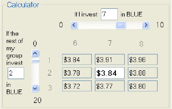
In addition to the practice rounds, subjects had access to a payoff calculator
throughout the tutorial and the experiment. The payoff calculator (Figure 3) allows
subjects to choose a hypothetical decision for themselves, a hypothetical combined
investment in the BLUE investment for the rest of the group, and provides information on
their payoffs under the current parameters, as well as the own-payoff consequences of
single-token changes in either direction for themselves or for the group. The practice
periods and tutorial were intended to introduce subjects to the decision task, familiarize
14
the calculator and the interface before making decisions for real payoffs. We collected
[image:28.612.109.391.127.306.2]data on the number of practice rounds each subject chose to use.
Figure 3. Payoff calculator
Once the experiment concluded, subjects were asked to fill out a questionnaire
while payments were prepared. This questionnaire included basic demographic data, as
well as data on education and measures of outlook regarding trust, justice, and human
nature.
Hypotheses
The primary hypotheses of interest are as follows ( indicates mean):
1. The Nash equilibrium outcome is a good predictor of subjects’ choices:
.
2. The Pigovian subsidy has the theoretically predicted effect:
, where is the mean investment in the CPR at the pre-subsidy social
3. The presentation of information has no effect: .
If subjects express other-regarding preferences—particularly pure, impure, or
paternalistic altruism—we should expect 1 and 2 to fail. In particular, if other-payoff
enters positively into the utility function, we should expect and
.
If subjects are intending to express other-regarding preferences, but making errors
in the attempt, the provision of information on the group payoff in addition to
information on their own payoff would allow them to change their investment decisions
to more accurately represent their preferences. If they possess an external norm that
indicates that, given an opportunity to make the group better off at one’s own expense,
one ought to take such an opportunity, provision of information on the group’s total
payoff provides both a reminder of the relevance of the choice task to group welfare and
information on how to improve group welfare at one’s own expense. Finally, if
information acts as a coordination point, even self-interested agents might strategically
coordinate on a point that would give them higher payoffs with the hope of either
sustaining a higher level of earnings or reneging in the future. Consequently, if subjects
are either prone to errors, have norms that are not fully internalized, or are prone to
strategic coordination, we should expect to see .
In addition, we test a number of other hypotheses regarding subsets of the data to
try to get a more accurate picture of subject behavior. We also consider other questions,
including the source and causes of deviations from Nash strategy, as well as concerns
16
Results
As previously mentioned, in both treatments the first seven rounds were baseline
rounds, as were the last seven rounds, with the intervening seven rounds presenting
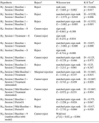
experimental treatments. We report the results discursively; statistical test results are
presented in Table 1 and indexed by hypothesis being tested (e.g. H1, H2, …). In the
table, ―Baseline 1‖ refers to periods 1-7, ―Baseline 2‖ refers to periods 15-21, and
―Baseline‖ without a number refers to the combined results from Baseline 1 and Baseline
2. In addition, unless otherwise specified, the variable of interest in this section is the
across-period mean CPR investment decision by a given subject, paired when
appropriate. This approach accounts for both individual and group fixed effects.
The sessions differ significantly (H1: p = 0.000, Figure 4). The mean baseline
investment in the CPR in Session 1 was 8.803 tokens, while the mean baseline
investment in Session 2 was 7.964 tokens. The null that these are equal can be rejected.
In addition, there is evidence of either learning or a ―decay‖-type trend (probably both).
In the first session, baseline 1 mean investment in the CPR was 8.517 (SE = 0.126)
tokens while the baseline 2 mean investment was 9.088 (SE = 0.063) tokens. Again, we
can reject the null of equality (H2: p = 0.010). In the second session, the baseline 1 mean
investment was 7.452 (SE = 0.200) tokens, while the baseline 2 mean investment was
8.476 (SE = 0.125) tokens. Once again, we can reject the null that these observations are
drawn from the same distribution. (H3: p = 0.003).
Figure 5 presents the mean decision by period in the first session. In the first
session baseline periods, we cannot reject the null that subjects’ behavior accorded with
Table 1. Statistical tests of hypotheses and robustness checks
Hypothesis Reject? Wilcoxon test K-S Test6
H1: Session 1 Baseline =
Session 2 Baseline
Reject rank-sum
Z = 3.665, p = 0.002
D = 0.4464, p = 0.017
H2: Session 1 Baseline 1 =
Session 1 Baseline 2
Reject matched-pairs sign-rank Z = -2.575, p = 0.010
D = 0.5238, p = 0.006
H3: Session 2 Baseline 1 =
Session 2 Baseline 2
Reject matched-pairs sign-rank Z = -3.002, p = 0.003
D = 0.3333, p = 0.093
H4: Session 1 Baseline = 9 Cannot reject sign-rank
Z=-0.863, p =0.388
H5: Session 1 Treatment = 6 Cannot reject sign-rank
Z=-0.233, p =0.816
H6: Session 1 Baseline =
Session 1 Treatment
Reject matched-pairs sign-rank Z = -3.002, p = 0.000
D = 0.857, p = 0.000
H7: Session 2 Baseline = 9 Reject sign-rank
Z=-6.714, p =0.000
H8: Session 2 Baseline =
Session 2 Treatment
Cannot reject matched-pairs sign-rank Z = 0.729, p = 0.466
D = 0.125, p = 0.975
H9: Session 2 Baseline 2 =
Session 2 Treatment
Reject matched-pairs sign-rank Z = 3.211, p = 0.001
D = 0.25, p = 0.347
H10: Session 2 Mid-Baseline =
Session 2 Treatment
Marginal rejection matched-pairs sign-rank Z = 1.416, p = 0.157
D = 0.1667, p = 0.815
H11: Session 2 Baseline 2 =
Session 2 Treatment (detrended)
Cannot reject matched-pairs sign-rank Z = 0.743, p = 0.458
D = 0.1667, p = 0.820
H12: Session 2 Mid-Baseline =
Session 2 Treatment (detrended)
Cannot reject matched-pairs sign-rank Z = 0.972, p = 0.331
D = 0.1667, p = 0.834
H13: Session 2 Baseline =
Session 2 Period 8
Reject matched-pairs sign-rank Z = 2.258, p = 0.024
D = 0.375, p = 0.047
H14: Session 2 Mid-Baseline =
Session 2 Period 8
Reject matched-pairs sign-rank Z = 2.733, p = 0.006
D = 0.417, p = 0.020
H15: Session 2 Baseline = 9
(random-effect tobit model)
Cannot reject Wald test
= 0.02, p = 0.896
6 Where appropriate, we use a boot-strapped (10,000 iteration) Kolmogorov-Smirnov test of equality of
18
Figure 4. Mean BLUE investment by period by session
(NE line indicates Nash equilibrium prediction without subsidy)
Figure 5. Investment decisions by period, Subsidy Session
treatment
0
1
2
3
4
5
6
7
8
9
10
1 7 14 21
Period
decision (no tax) decision (tax)
mean decision by period
D
e
ci
si
o
[image:32.612.110.472.409.673.2]the effect posited by Pigou (H5: p = 0.816). Subjects’ mean investment in the CPR was
5.946 (SE = 0.154) tokens, which is not significantly different from the Pigovian
prediction of 6 tokens. We can reject the null of no treatment effect; this is robust to using
the first, the second, or the combined baseline treatment as a basis for comparison (H6: p
= 0.000).
Because of the existence of an underlying time trend, two approaches were used
to try to separate the effects of learning and decay from the treatment effect. The first is
to use as a basis of comparison only those periods which are most like those of the
treatment group in terms of learning and decay—namely, the last three of the first
baseline and the first four of the second baseline, which we will refer to as the
―mid-baseline.‖ Using the mid-baseline has a few advantages: we expect some of the noise of
experimentation and learning has dissipated by period 5, while these periods do not
contain the same level of decay as the last three periods.
The second attempt requires the assumption of a linear trend that is stationary
throughout the session. Elimination of this trend was done by simple OLS regression of
the subjects’ investment decisions on the period, and then subtraction of this period-based
component to produce a de-trended decision. For the subsidy treatment session, neither
method has a qualitative effect on the magnitude or significance of this treatment effect.
For the second session, we can reject the null that pooled baseline behavior is
equal to the Nash prediction (H7: p = 0.000), and subjects’ investment decisions appear to
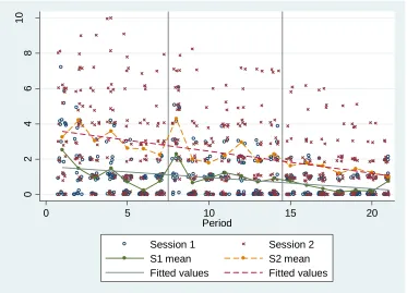
be noisier and converge later than do those in the first session (Figure 6). The effect of
the information they receive is more difficult to discern. The mean contribution decision
20
reject the null of equality with the baseline mean (H8: p = 0.466). Considering the
dispersion of decisions in the first several periods of this session, however, other tests
seem appropriate. Comparing the treatment periods only to the second baseline, for
example, produces a paired test that recommends rejecting the null of equality (H9).
Because the treatment precedes this second baseline, it appears that the underlying
time-trend may confound the result. Both methods to account for the time-time-trend in the first
[image:34.612.109.472.265.524.2]session were also used for the second session.
Figure 6. Investment decisions by period, Information Session
The mean contribution in the mid-baseline periods was 8.125 (SE = 0.162), which
is marginally different than that of the treatment group (H10). The mean de-trended
decision in the session was 7.127 (SE = 0.117) tokens in the CPR. Use of the de-trended
version removes any significant difference between the second baseline and the treated
group or the mid-baseline and the treated group (H11, H12).
0 1 2 3 4 5 6 7 9 8 10
1 7 14 21
Period
decision (no info) decision (info)
mean decision by period
A sharp decline in contributions is visible in Figure 6 during period 8, the first
period of the treatment (mean contribution to the CPR = 6.750, SE = 0.494).
Nonparametric tests indicate that this is indeed significantly different from the full
baseline, as well as the mid-baseline, and that these results persist even in the de-trended
data (H13, H14).
It is unclear that an assumption of a linear trend is a legitimate one, so while the
tests for the de-trended data are illustrative, they may not be conclusive. A more
sophisticated test for an effect of information can be developed by considering the nature
of the treatment: in particular, subjects may see one of three different types of message.
For subjects in groups that under-invest in the CPR, they are informed that an increase in
their level of investment would increase the payoff to the group. For those in groups at
the social optimum, they are informed that their current level of investment is optimal.
Finally, for those in groups suffering from overcongestion in the CPR, subjects are
informed that a reduction in investment would lead to an increase in group payoff. It may
be the case that the information is having an effect, but that offsetting behavior leads to
an inability to reject the null of no effect, because the changes preserve the mean level of
investment within subjects.
In practice, of the 168 messages subjects received during the information
treatment, 147 informed subjects that a decrease would improve group payoff, 9 informed
subjects that an increase would improve group payoff, and 12 informed subjects that they
were at the maximum group payoff. Consequently, 12.5% of the messages sent to
subjects would not be expected to induce a reduction in CPR investment. Considering the
22
should allow a better test of a treatment effect. Consider this ―sub-treatment‖ the
―Decrease‖ treatment.
Selection of the counterfactual is important in this case. Those who received the
Decrease treatment are similar in known ways. First, these are subjects in the Information
session. Second, the decisions under the treatment occur during the middle seven periods.
Finally, only those who were members of groups whose combined investment in the
previous period exceeded the socially optimal level of investment received advice to
decrease their investment. For a basis of comparison, we can consider decisions that meet
the first and third criteria as ―candidates for treatment.‖
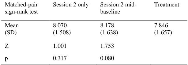
Considering all periods in session 2, we cannot reject the null of no effect of the
Decrease treatment (Table 2). When comparing against the mid-baseline, we can reject
the null of no effect at the 10% level. In both cases, these hypothesis tests are
unconditional and, as we are using mean levels of investment by subject, we have 24
observations. Using regression methods, we may be able to account for censoring and
[image:36.612.170.477.519.625.2]improve statistical power.
Table 2. Tests of the effect of the Decrease treatment
Matched-pair sign-rank test
Session 2 only Session 2 mid-baseline Treatment Mean (SD) 8.070 (1.508) 8.178 (1.638) 7.846 (1.657)
Z 1.001 1.753
p 0.317 0.080
In this case, again, selection of the counterfactual is important. In order to
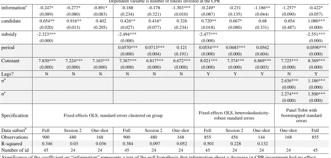
Table 3 presents the results for selected regressions. Those observations that are
considered ―candidates‖ from session 1, under the ―Full‖ subset of the data, are those
investment decisions for which the group decision in the previous period exceeded the
social optimum and the price level was the same as in the information treatment in both
the preceding period and the period in which the decision was made. The reported results
are robust to modifications in the chosen counterfactual set of observations.
In addition to tests of the average effect of the Decrease treatment over the
seven-period treatment, the regressions include specifications using only the first 8 seven-periods of
session 2 (the results labeled ―One-shot‖ in the ―Data subset‖ row), which provides a test
of the effect of the Decrease treatment on first sight. This ―first-sight‖ effect is always
significant at the 10% level. Subjects’ observed choices declined significantly the first
time they received the Decrease treatment.
The effect of the Decrease treatment is always negative and generally significant,
so this particular form of information provision appears to have a small negative effect on
investment in the CPR that spikes in subjects’ first exposure, reducing investment levels
on average by a little over a single token, but which does not persist through subsequent
periods. It is smaller than the effect of the Pigovian subsidy, but is perhaps surprisingly
large, given that there is no direct appeal to social norms nor any communication allowed
among subjects. These results represent a roughly 9% increase in subjects’ single-period
earnings as a result of the first exposure to the Decrease treatment, indicating that there
may be greater efficiency gains possible without requiring a costly intervention such as a
24
Table 3. Regression results under different specifications
Dependent variable is number of tokens invested in the CPR
informationa -0.247* -0.277* -0.891* -0.188 -0.178 -1.303*** -0.249* -0.231 -1.186** -1.257* -0.422* (0.089) (0.080) (0.083) (0.234) (0.321) (0.010) (0.087) (0.135) (0.044) (0.090) (0.057)
candidate 0.654** 0.916** 0.402 0.426** 0.416* 0.326 0.720** 0.667* 0.68 0.654 1.080***
(0.020) (0.013) (0.205) (0.027) (0.077) (0.234) (0.018) (0.080) (0.331) (0.487) (0.000)
subsidy -2.323*** -2.494*** -2.477*** -2.551***
(0.000) (0.000) (0.000) (0.000)
period 0.0570*** 0.0713*** 0.121 0.0554*** 0.0683*** 0.0562 0.0590***
(0.000) (0.004) (0.191) (0.000) (0.000) (0.604) (0.000) Constant 7.830*** 7.224*** 7.163*** 7.367*** 6.817*** 6.672*** 8.021*** 7.374*** 6.869*** 7.725*** 8.369***
(0.000) (0.000) (0.000) (0.000) (0.000) (0.000) (0.000) (0.000) (0.003) (0.000) (0.000)
Lags? N N N N N N Y Y Y N Y
σu
2.636*** 1.186*** (0.000) (0.000) σe
2.274*** 1.500*** (0.000) (0.000)
Specification Fixed-effects OLS, standard errors clustered on group Fixed-effects OLS, heteroskedasticity-robust standard errors
Panel Tobit with bootstrapped standard
errors Data subsetb Full Session 2 One-shot Full Session 2 One-shot Full Session 2 One-shot One-shot Full
Observations 900 480 168 900 480 168 855 456 144 168 855
R-squared 0.346 0.03 0.036 0.384 0.097 0.052 0.501 0.228 0.132
Number of id 45 24 24 45 24 24 45 24 24 24 45
a
Significance of the coefficient on ―information‖ represents a test of the null hypothesis that information about a decrease in CPR investment had no effect.
b
―Full‖ indicates both sessions are included with the first period omitted, as candidacy for treatment depends on lagged group decisions. ―Session 2‖ indicates only session 2 data is included. ―One-shot‖ indicates that data is drawn from periods 1 – 8 only.
The observed difference between sessions may be correlated with use of practice
rounds. During the tutorial phase of the experiment, subjects had the opportunity to play
with a deterministic computerized ―rest of the group‖ as many times as they liked. The
median number of practice rounds for subjects in Session 1 was 3.5, while the median for
session 2 was 1.5 (the corresponding means are 9.04 and 5.583). The two distributions
are marginally significantly different (the Mann-Whitney test gives a p-value of 0.1215,
but the total number of subjects is only 45), but in other observable ways, the two
sessions appear to draw from the same population.7
This seems to be borne out by the progress of subjects’ behavior over the course
of the experiment. The mean absolute deviation from best response is, in a sense, a
measure of the deviation from self-interested behavior, as payoffs are decreasing with
this deviation. Figure 7 presents the mean absolute deviation from the best response over
time: it is clear that both samples are converging over the course of the experiment—in
the limit, to the Nash prediction—but that 21 periods are not enough to ultimately
converge within the second session.
If learning is a concern, we might expect the practice rounds to help subjects
converge, and indeed there is a marginally significant effect of the number of practice
rounds played on the mean absolute deviation from best response (p=0.058, n = 45). For
the average subject, in terms of mean absolute deviation from best response, the effect of
practice rounds reduces the mean absolute deviation from best response by 0.0354 tokens
7 An early hypothesis for the difference in baseline behavior was a ―Friday effect,‖ as the second session
26
per round. With an average number of tutorial trials of 7.18 across the full sample, the
mean effect of practice rounds reduces the mean absolute deviation from best response by
[image:40.612.110.483.154.423.2].25 tokens, or a 15% reduction in average absolute deviation.
Figure 7. Absolute deviation from best-response by period by session (with population means and lines of best fit)
Conclusion
As population continues to rise, the impact of congestion externalities continues
to increase. Common-pool resources are increasingly policy-relevant, and while there is a
growing literature on common-pool resource experiments, these goods still have not
received the research attention that private and pure public goods have received. The
reasons for this are both technical and theoretical—these goods are complicated by their
very nature, and the institutions that govern them vary widely. This experiment presents a
simplified common-pool resource experiment to subjects and the results indicate that
0 2 4 6 8 10 a b s( d e lt a b r)
0 5 10 15 20
Period
Session 1 Session 2
S1 mean S2 mean
subjects do indeed converge to the Nash prediction under these conditions, but that
convergence can take quite a while.
One of the simplest (theoretically, if not practically) policy tools to correct for the
congestion externality inherent in common-pool resources is the introduction of a
Pigovian tax or subsidy to internalize the externality. We show that such an intervention,
if feasible, should have the effect hypothesized by Pigou. Bearing in mind the
impracticality or high cost of introducing such a direct intervention, we find a smaller,
but significant effect from an information provision treatment. Further study on similar
approaches to appeals to social norms should provide more insights into how effective
such appeals can be at reducing congestion in common-pool resources. Ferraro (2009),
for example, reports a large-scale randomized policy field experiment and finds that
―pro-social‖ messages have an effect on water use. The information treatment used here
primarily provides information, rather than appealing directly to social norms. Future
research should look at the effect of specific appeals to social norms in reducing
congestion in the lab.
In addition, extending the experiment to incorporate taxes directly, allowing
subjects to see marginal changes in both own- and other-payoff, changing group size, and
directly modifying marginal per-capita return on investment would provide useful
information on the sensitivity of CPR consumption decisions to these conditions. In
particular, experiments using very large groups could be useful in extending external
validity to more closely represent naturally occurring common-pool-resources.
Finally, we find that subjects’ participation in practice rounds has a positive and
28
evidence on the rate of subjects’ convergence to equilibrium, confirms that common-pool
resource experiments are complicated, and our inference with respect to subject behavior
Chapter II: Apples to Apples to Oranges
Fiscal Need in the United States in a Regression-Based Representative Expenditure Approach
Introduction
Fiscal need is a measure of the ability of a sub-national government (SNG) to
provide an average level of services with an average level of revenue. The level of
services required of U.S. states has grown over the last fifty years, without reference to
the differing abilities of the states to keep up with these requirements.8 The latter half of
the twentieth century witnessed the steady advance of minimum standards of public
service provision, motivated both by local public choice and by federal legislation.
Such laws, in general, have the potential to create efficiency gains. The federal
government has the unique ability to internalize externalities at the national level,
circumventing difficult public choice quandaries that can lead to pollution havens or
interstate competition over fair labor standards, for example. While many programs have
been designed and mandated at the national level, the fiscal apparatus required to
implement them, including the primary source of funding, remains primarily a state and
local phenomenon: national standards are not generally funded by the Federal
Government (e.g. No Child Left Behind and the Clean Air Act). States face different
challenges in complying with these standards. A state with a stiff wind blowing in off the
coast may find it easier to comply with clean air standards, while a state with entrenched
8 Since 1960, the share of GDP devoted to state and local public expenditure has nearly doubled from
30
poverty and low levels of adult education may have a difficult time improving
eighth-grade test scores.
A common standard with heterogeneous costs and needs leads to spending
different amounts of money to provide a mandated level of public services. Implicitly,
this results in redistribution of net fiscal burden (NFB) across states. The fiscal
equalization literature notes that redistribution represents an opportunity to advance both
equity and efficiency through equalization. By the same token, service provision
standards without consideration of fiscal need can reduce both efficiency and equity.
The implications for policy have an upside: policy that accounts for this
burden-shifting can improve efficiency and equity by eliminating the incentive to move for fiscal
reasons. In principle, this means equalizing the NFB for each individual across SNGs. In
practice, the policy goal has been to provide SNGs with the ability to do so by equalizing
―fiscal comfort,‖ or the ability of a SNG to provide an average level of services with an
average level of tax effort, not revenue.
Measuring fiscal comfort involves measuring two dimensions: revenue-raising
ability, or ―fiscal capacity,‖ and service-provision ability. Measuring fiscal capacity has
proven to be more straightforward than measuring fiscal need for practical, theoretical,
and analytical reasons, and as a result most equalization schemes are based on tax
equalization.9 This adjusts revenue as though per-capita expenditure need were constant
within a country. When only tax treatment is accounted for in an equalization program,
the equalization program may increase efficiency, but there remains an incentive to move
to reduce one’s NFB, and thus allocative inefficiencies remain (Boadway and Flatters
1982). Tax-based equalization leaves money on the table.
Empirical evidence indicates that ignoring fiscal need is economically significant.
Wilson (2003) looks at Canadian migration data in response to Canada’s capacity-based
equalization program and finds significant efficiency gains in addition to the more
straightforward equity improvements. Shah (1996) provides evidence on the size of the
disparity that arises from excluding fiscal need in Canada’s equalization program and
finds that incorporating expenditure need in the measure of fiscal comfort leads to
significant changes in the existing entitlements, nearly halving the net transfer out of
Ontario and nearly doubling the net transfer out of British Columbia.
Given the potential gains from a fiscal-comfort approach, why do existing policies
generally ignore fiscal need? There are several reasons. First, the concept of fiscal need
can be politically unpalatable. As controversial as property value assessments can be, the
idea of measuring a tax base is relatively straightforward. Asserting that higher levels of
per-capita expenditure in one area are ―necessary‖ or ―just,‖ while it advances equity in
practice, may appear to violate the principle of equity.10 In addition, this policy approach,
like others, creates winners and losers relative to the status quo. Any change is likely to
be met with resistance from those who lose from the policy change, even if net social
welfare is improved.
Second, while the size of the tax base does not directly depend on preferences, the
size and structure of public expenditures does, and so differentiating between
idiosyncratic preferences for public goods and fiscal need must be done by assumption or
10
32
by government definition. As is often the case, our estimates must be qualified by these
assumptions, or by the adequacy of government guidelines.
Finally, measurement of fiscal capacity runs into problems typical of
measurement of stocks and flows of capital, while fiscal need measurement requires a
more diverse set of variables: people and their possessions, the stock of existing public
infrastructure, crime rates, public health measures—any major determinants of public
expenditure.
Despite these challenges, the literature has sought to develop some good measures
of fiscal need. The primary approaches to measuring both fiscal capacity and fiscal need
were developed by the Advisory Committee on Intergovernmental Relations (ACIR).
Mushkin and Rivlin (1962) developed the Representative Tax System (RTS) to measure
fiscal capacity, and Rafuse (1990) introduced the complementary Representative
Expenditure System (RES) to measure fiscal need. In both cases, the approach uses mean
values across SNGs as the benchmark to which all SNGs are compared, and produces
absolute levels of capacity or need as well as an index for comparison across SNGs.
The RTS approach has become well-established, but the RES approach has seen
less use. Most noteworthy is the contribution of Robert Tannenwald, who produced a
series of papers continuing and improving on Rafuse’s RES approach (Tannenwald 1999;
Tannenwald and Cowan 1997; Tannenwald and Turner 2004; Yilmaz, Hoo, Nagowski,
Rueben and Tannenwald 2006). The existing work using the RES method has relied on
Rafuse’s original workload-based approach which, while informative and parsimonious
with respect to data, relies heavily on assumptions in generating its estimates of fiscal
states as the unit of analysis and finds that the estimates are sensitive to variables selected
for inclusion. Boex and Martinez-Vazquez (2007) note that ―the technically most
sophisticated techniques (notably local expenditure needs computed using a
regression-based [RES])…quite possibly provide the best possible measures.‖ (p. 329). If this is the
best measure, why is it not more widely implemented? Bird and Vaillancourt (2007)
provide some insight:
Almost all who have studied the RTS-RES approach agree on two points: first, it is formally the most satisfactory way to meet the normative objectives of the theoretical equalization model, and, second, that it is difficult and costly to obtain the necessary data…, especially for expenditures. (284)
This is certainly the case in many of the countries Bird and Vaillancourt consider.
Data in the United States is readily accessible, however, and these data make it possible
to explore the differences between workload- and regression-based approaches, as well as
the practical data requirements for improving regression-based estimates.
In addition, these representative approaches rely on the assumption that observed
patterns of revenue and expenditure accurately capture decisions made by autonomous
local governments in raising revenue and providing services to meet the needs of their
constituents. To the extent that observed patterns instead represent structural
inefficiencies from central control, discrimination across segments of society, or factor
immobility, for example, both the RTS and RES would fail to correct for these historical
problems. This is unlikely to be the case in the United States, but any implementation of
an RTS-RES approach should consider these possible problems.
This paper represents several contributions to the literature. First, we introduce a
―hybrid-regression‖ method of determining fiscal need. Using this method, we make use
34
where relevant) or the surrounding rural areas (hereafter referred to as a group as
―sub-state areas‖). We produce per-capita need measures by sub-―sub-state area. Next we use this
data to generate measures of fiscal need for SNGs, which include the fifty states and the
District of Columbia. We thus contribute to the public finance and urban and regional
economic literatures by producing the first MSA-level and sub-state-level measures of
fiscal need for the United States as well as the first regression-based measures of fiscal
need for states (including D.C.).11 Finally, we produce estimates using other
regression-based methods with different levels of data aggregation and different levels of data
availability for comparison.
We find that estimates of need depend on the approach used to estimate need
levels. These estimates differ greatly from previous workload-based approaches,
consistent with previous comparisons of regression- and workload-based estimates (Boex
and Martinez-Vazquez 2007). The preferred estimates are relatively robust across
regression-based approaches, maintain a U-shaped trend with respect to population
density, and accord more closely with actual expenditure than previous estimates.
Sub-state-level estimates also indicate that while the District of Columbia is an
outlier among states, it is not unique among cities (Delaney 2007). Comparing measures
developed with state- and sub-state-level data reveal high correlation. However, the use
of state-level data significantly and systematically overestimates need in larger, less
populated states, relative to the more disaggregated approach.
11 Previous regression-based RES estimates exist for the provinces of Canada (Shah 1996) as well as the
Cost and Comparability in States and Cities
The RES method runs into several complications, which we refer to as
comparability and cost. Figure 8 presents actual per-capita direct expenditures in the
United States and illustrates the comparability issue: when developing relative measures
and transforming them into absolutes, one must establish comparable jurisdictional units.
The District of Columbia, Alaska and Hawaii provide obvious examples of idiosyncratic
SNGs, although the same critique applies to many interstate comparisons. Looking at
data from the 2002 Census of State and Local Government Finances, public expenditure
varies across states, with direct per-capita expenditures in 2002 ranging from $4,746 in
Arkansas to $10,802 in Alaska (Figure 8). In principle, actual expenditures should be
positively correlated with expenditure need, but measuring disparity is difficult without
[image:49.612.112.546.412.597.2]accounting for heterogeneity.
Figure 8. Per-capita state-and-local direct expenditure by state in 2002 ($1,000)
States vary widely across a number of dimensions, including land area,
population, urbanization, land rents, industrial characteristics, input costs, prices of final