Georgia State University Georgia State University
ScholarWorks @ Georgia State University
ScholarWorks @ Georgia State University
Real Estate Dissertations Department of Real Estate
Summer 7-23-2010
Agricultural Commodity Futures and Farmland Investment: A
Agricultural Commodity Futures and Farmland Investment: A
Regional Analysis
Regional Analysis
John S. Clements III
Georgia State University
Follow this and additional works at: https://scholarworks.gsu.edu/real_estate_diss
Recommended Citation Recommended Citation
Clements, John S. III, "Agricultural Commodity Futures and Farmland Investment: A Regional Analysis." Dissertation, Georgia State University, 2010.
https://scholarworks.gsu.edu/real_estate_diss/8
This Dissertation is brought to you for free and open access by the Department of Real Estate at ScholarWorks @ Georgia State University. It has been accepted for inclusion in Real Estate Dissertations by an authorized
1
In presenting this dissertation as a partial fulfillment of the requirements for an advanced degree from Georgia State University, I agree that the Library of the University shall make it available for inspection and circulation in accordance with its regulations
governing materials of this type. I agree that permission to quote from, or to publish this dissertation may be granted by the author or, in his/her absence, the professor under whose direction it was written or, in his absence, by the Dean of the Robinson College of Business. Such quoting, copying, or publishing must be solely for scholarly purposes and does not involve potential financial gain. It is understood that any copying from or publication of this dissertation which involves potential gain will not be allowed without written permission of the author.
2
Notice to Borrowers
All dissertations deposited in the Georgia State University Library must be used only in accordance with the stipulations prescribed by the author in the preceding statement. The author of this dissertation is:
John Sherwood Clements III 300 Peachtree Street NE, Unit 11A Atlanta, Ga. 30308
The director of this dissertation is:
Dr. Alan J. Ziobrowski Real Estate
P.O. Box 3991 Atlanta, Ga. 30302
Users of this dissertation not regularly enrolled as students at Georgia State University are required to attest acceptance of the preceding stipulations by signing below. Libraries borrowing this dissertation for the use of their patrons are required to see that each user records here the information requested.
3
Agricultural Commodity Futures and Farmland Investment: A Regional Analysis
BY
John Sherwood Clements III
A Dissertation Submitted in Partial Fulfillment of the Requirements for the Degree of
Doctor of Philosophy
in the Robinson College of Business of
Georgia State University
GEORGIA STATE UNIVERSITY ROBINSON COLLEGE OF BUSINESS
4 Copyright by
5
ACCEPTANCE
This dissertation was prepared under the direction of the candidate’s Dissertation
Committee. It has been approved and accepted by all members of that committee, and it has been accepted in partial fulfillment of the requirements for the degree of Doctor in Philosophy in Business Administration in the Robinson College of Business of Georgia State University.
H. Fenwick Huss Dean
Robinson College of Business
6 ABSTRACT
Agricultural Commodity Futures and Farmland Investment: A Regional Analysis By
John Sherwood Clements III July 23, 2010
Committee Chair: Dr. Alan J. Ziobrowski
Major Department: Real Estate
Using seventeen years of data from 1991 to 2008, I derive a pricing model for farmland values. This valuation model is the first using agricultural commodity futures as a proxy
for “ex ante” income projections for the crops grown or livestock grazed on United States farmland. While not all inclusive, the model is tested regionally including the Corn Belt, Delta States, Lake States, Mountain, Pacific Northwest, Pacific West and Southeast
Regions. Additionally, I test whether interest rate futures contracts have a relationship with farmland values as interest rates have been proven to be a reliable predictor in past
research. Farmland capitalization rates and anticipated inflation have hypothesized relationships, but are mainly used as control variables in the study.
In general, agricultural commodity futures contracts are a poor predictor of changes in farmland market values. When examining relationships with quarterly percentage change
7
futures prices have a significant relationship with farmland values in the Corn Belt region. Interest rate futures contracts, farmland capitalization rates and anticipated
inflation are not statistically significant in the majority of the regions.
As a robustness check, I model the price levels of the variables using Johansen’s cointegration procedure. This time-series econometric methodology provides results in regards to long-run equilibrium relationships between the variables. The results are only
slightly better. Corn, orange juice and sugar futures contracts have positive statistically significant relationships with farmland market values in multiple regions. Again, wheat
8
Acknowledgements
I would like to dedicate this dissertation to my immediate family who provided me the support to continue down this challenging path of obtaining a doctoral degree. My mother, Mary Frances Page Clements provided the emotional and financial support
necessary to withstand the challenges that stood in the way. My sister, Mary Page Clements showed me that dreams could become a reality by firmly entrenching herself in
theatrical education in New York City. My late father, John Sherwood Clements, Jr. instilled the notion that real estate education is an admirable avenue for success and I am sure he is looking down upon me with satisfaction this very day.
I would like to thank the my dissertation chair, Dr. Alan Ziobrowski for being not only
my guide throughout the doctoral process, but my friend that provided constant encouragement as well as constructive criticism. I also appreciate the department chair, Dr. Julian Diaz as he in my opinion set the standard for what I should attempt to become
through the way he lives his daily life as well as his dedication to real estate research of which very few have dared to embrace. Additionally, I would like to thank the other
professors that either provided advice or disseminated knowledge that allowed me to complete my dissertation. These people included Dr. Paul Gallimore, Dr. Edward Rigdon, Dr. Karen Gibler, Dr. Joseph Rabianski, Dr. Gerald Gay, Dr. Shelton Weeks, Dr.
9
I would like to express gratitude to my colleagues that have become lifelong friends throughout the adventure that is a doctoral degree. These include Alan Tidwell, Vivek
Sah, Xiaorong Zhou, Frank Gyamfi-Yeboah, Changha Jin, Seunghan Ro, Phil Seagraves, Julia Freybote, Preshant Das and Alan Ferguson. Also, I am grateful for the people that
stood behind me with friendship as I left Thomson, Georgia to follow my dream of attaining the doctorate in real estate at Georgia State University. These are Todd Ingram, Dexter Lovins, Douglas Pentecost, Butch Stadler, Phillip Farr, Faye Knighton, Boone
Knox, Terry Barber, Robert Campbell and Mike Shirah.
10
Chapter One
Introduction
Agricultural commodity production has increased in efficiency in recent years due to advances in technology in harvesting, equipment, and processes. Farmland has provided
record returns, including appreciation (depreciation), income (losses) and realized capital gains, over the past 5 years outperforming other asset classes such as stocks, bonds, offices, and apartments (Newell and Eves, 2007). Yet, farmland is arguably one of the
least transparent real estate investment classes, thus utilization by institutional investors is lacking compared to other assets. Pricing models and the valuation of farmland have
been the topics of numerous studies in past research and one central theme is the differing choice of variables used in these studies. My research integrates the futures market into the process of pricing this unique asset class of our economy.
Farmland makes up a significant portion of the real estate asset market in the United
States. As of 2007, the number of farms in the United States totaled 2,204,792 and with an estimated value of $1,744,295,252,000 (USDA, 2007). According to the USDA, the value of farmland increased approximately 50% from 2002-2007. The average price per
acre increased from approximately $1200 an acre to nearly $1900 an acre during this timeframe. In the United States, approximately 29,000 farms are held by institutional
11
Investment in farmland has also increased as a result of the enactment of the Employment Retirement Income Security Act in 1974. This law required pension funds to diversity
their portfolios. Investments like timberland and farmland that were often overlooked in favor of stocks and bonds became attractive options for these institutions. Large
institutional investors such as Hancock Agricultural Resource Group, UBS Agrivest, and even the Mormon Church are among the most prominent large scale investors in farm assets. Farmland investment by institutional investors, corporations, partnerships, and
others is 13.5% of the total farmland economy with approximately 348,000,000 acres (USDA, 2007).
Asset Valuation
The fundamental value of any financial asset is the present value of expected future cash
flows (Brigham and Daves, 2004). An asset is valued by forecasting the expected cash flows and discounting these flows over the holding period by a required rate of return
(Discounted Cash Flow model or DCF). This model can be used for stocks, bonds and even real estate. Real estate and other financial assets may also be valued with relative value models. These are data-based approaches where historic transactions of similar
assets in the same market are examined to derive a market value estimate (Knight, Sirmans, and Turnbull, 1998). A third valuation model of financial assets including real
12
future development or change of use, but the chance of immediate development decreases with this greater uncertainty.
For the purposes of this study, I consider the valuation model for farmland to be a present
value model. The model is not DCF, but uses similar finance theory as farmland value is based upon the expectations of income produced by farm commodity products. These expectations are taken from the futures markets, which provide daily trading of futures
contracts used for speculation of commodity prices to hedge downside risk.
Farmland Pricing Model
Pricing models for various investments such as stocks, bonds, commodities and farmland have been examined extensively in prior research. Consistent with finance theory, Falk
(1991) notes that when markets have rational expectations and constant discount rates, the present value of expected current and future real net rents produced by a tract of
farmland at the end of a given time period should be equal to the real farmland prices at the beginning of that time period. However, Shiller demonstrates, using other assets, this relationship is inconsistent with the observations of real markets. Shiller (1979) shows
that bond yield volatility is too large when based only on changes in the term structure of interest rates. Similar, Shiller (1981) evaluates the classic valuation model for stocks and
finds that stock price volatility is too large to be explained solely by the present value of future dividends. Further, Case and Shiller (1989) find evidence that is consistent with the notion that real estate is inefficient as well. They find that predictable movements in
13
markets of Atlanta, Chicago, Dallas, and San Francisco. The authors add that rents cannot truly be measured by differences in the quality of construction of rental and owner
occupied housing, so the question of market efficiency is not definitively answered in their study.
Shiller (1984) argues that social dynamics he calls “fads and fashions” are important in assessing the movements of speculative asset prices. He shows, for example, that stock
prices consistently overreact to new information on dividends. Thus asset prices cannot be forecast strictly on the basis of present value of future cash flows. Different types of
assets may be “fashionable” (intrinsically more valuable) at some times and “unfashionable” at other times. Falk (1991) provides other arguments after testing the Efficient Market Hypothesis (EMH) on farmland prices. The null hypothesis of market
efficiency is rejected for Iowa farmland data and he proposes that farmland may have rational bubbles.
Farmland present value models have been tested extensively and most have rejected the model because of excess volatility in the real estate values as compared to income
measures such as cash rents (see Burt (1986), Falk (1991, 1992), Featherstone and Baker (1987), Tegene and Kuchler (1991, 1993), Hanson and Myers (1995), Engsted (1998),
14
reject to the PVM on all tests using 6% transaction costs and the authors considered this percentage to be more realistic for farmland.
Prior research does not include agricultural commodity futures as an explanatory variable
in their present value models and has provided a gap in the present farmland valuation literature. The dissertation’s main purpose is to bridge this gap in the literature. This is important as futures have provided farmers with the opportunity to hedge downside risk
since March 13, 1851 when the 1st recorded forward contract was introduced in Chicago, Illinois (Kline, 2000). In 1865, the 1st standardized futures contract was written by the
Chicago Board of Trade (Barrie, 2001).
Agricultural Commodity Futures
Real estate research using futures contracts in pricing models is very limited (See Hinkelman and Swidler (2008), Bertus, Hollins, and Swidler (2006), Clements,
Ziobrowski and Holder (2010), Liang, Seiler, and Chatrath (1998) and Jensen, Johnson and Mercer (2000). These studies test the usefulness of futures contracts as a hedging mechanism for such items as house price risk or REIT price returns, test the relationship
between lumber futures and timberland market values or test whether futures contracts can be held as a portion of an optimally diversified portfolio. Futures prices have been
15
For the purposes of this study, agricultural commodity futures are used as expectation of future income from the real estate asset farmland. Commodities used include annual row
crops, permanent trees, and livestock grazing on the land. Nationally, agriculture sales are split as crops and trees accumulated 48% with livestock adding the remaining 52%
(USDA, 2007). The five individual commodity leaders were: Cattle (21%), Corn (13%), Poultry (12%), Dairy Cattle (11%) and Soybeans (7%). It should be noted that not all commodities produced on farms are sold on the futures exchanges. Poultry, for example,
is not a commodity available for trading. Futures provide expectations of prices, while the spot prices are actual current prices on these commodities. Consistent with
expectations, as these futures prices rise the value of the land that produces these commodities should increase in the region that the crop is produced. I hypothesize that commodity futures should be positively related with farmland values in study.
Rationale and Scope of the Study
Farmland market values are the focus of the study and are derived from index data provided by the National Council of Real Estate Investment Fiduciaries (NCREIF). NCREIF is the largest agriculture index in the United States as it contains approximately
208 properties as of January, 2009 presently valued at over 1.1 billion dollars. NCREIF derives a nationally quarterly return index as well as geographic regions similar to the
annual Census of Agriculture published by the United States Department of Agriculture. My other focus, agricultural commodity futures are traded on the United States futures exchanges such as the Chicago Mercantile Exchange, Intercontinental Exchange, Kansas
16
C Research, Inc., a data mining company and includes all intra-day and end of day for most commodity futures available.
The sample period for the study is 1991 to 2008. I test ordinary least-squares regression
analysis on the percentage change in farmland market values as compared to the percentage change in the prices for agricultural commodity futures over the time period. In view of the rejection of the PVM, our models test additional variables such as
capitalization rates, interest rate futures, and anticipated inflation. Variables included in previous studies are interest rates, government payments, transaction costs, property
taxes, ex-post land and building returns, soil characteristics, commodity transportation costs, inflation and debt payments. Because of small sample size, I do not include all of the above mentioned variables in the model. Other methodologies such as regression
analysis on price levels and Johansen’s cointegration technique are used. I find support for my hypothesis if the futures prices and anticipated inflation have positive signs and
statistically significant with respect to farmland market values. Interest rate futures and farmland capitalization rates would be expected to have an inverse relationship with farmland market values.
Location is one of the most important factors in valuing real estate assets. Farmland is no
different as many agricultural commodities are location specific varying by climate and temperatures. I test farm products used in the study by region. The regions are the Pacific West, Pacific Northwest, Corn Belt, Delta States, Southeast, Mountain, Southern
17
and California; therefore we expect orange juice futures to have a significant positive relationship with farmland values in the Southeast and Pacific West regions. Similarly,
rough rice is grown in the Delta States region including Arkansas and Louisiana and we expect those futures prices to have a significant positive relationship with land values in
this region. National indexes are provided by NCREIF and I test each agricultural commodity future’s relationship with this index as well.
My study extends the current literature in several ways. First, the study uses agricultural commodity futures as an “ex-ante” component of the income produced from farmland.
This research provides a theoretical link to the expected income from crops growing and livestock grazing on the land. Phipps (1984) observes that returns in prior research are based upon income from operations using “ex-post” data and lagged to set up “ex-ante”
expectations relationship. I do not expect ante” futures values to be related to “ex-post” spot prices for the commodities, so our study extends the literature as it is forward
looking. Commodities are volatile and should be based upon future expectations per finance theory. I do not know if investors look at futures with regards to farmland investing and the study tests the hypotheses as to whether short-term futures prices do
indicate long-term trends as indicated by changes in farmland values.
Secondly, while farmlands have been studied on a regional basis as shown by studies by Moss (1997), Livanis, Moss, Breneman and Nehring (2006) and Mishra, Moss and Erickson (2008), they have not provided “ex-ante” income components attributable to
18
provide. Examples were given for orange juice and rough rice futures, but even futures such as live cattle that are found in all regions can be tested to see if commodity futures
prices are significant with respect to the location where they are grown or grazed. Third, prior research on farmland has shown interest rates to be a credible explanatory variable,
but have not used interest rate futures as an explanatory variable. Interest rate futures provide expectations of the change in interest rates over the short-term, similar to the agricultural commodity futures that provide expectations of the change in spot prices of
the commodity.
Lastly, past research using futures and real estate aimed at hedging risk. This study provides information for use with speculation and price discovery, which are two other typical reasons for entering and trading in the futures market. Theoretically, owners of
farmland in specific locations can examine prices for agricultural commodity futures and speculate on rising land values. The information provided by the futures may help with
decisions on land expansion, lease-purchase conversions, or sales of excess land.
The results of the study are intended to provide conclusions for “large farms” similar to
the farms located in the NCREIF index. NCREIF (2009) readily admits their portfolios represent a single asset class and may not represent the total agriculture market in the
19 Findings and Organization of Dissertation
In general, I find a weak relationship between agricultural commodities futures prices and farmland value. But in almost all regions of the United States, I find at least one
commodity whose price is significantly related to farmland value. In the quarterly regression models, the Mountain region had the most accurate pricing model, with, live cattle, Minnesota wheat and cotton futures being significant. In the long-run
cointegration models, sugar, corn and orange juice are significant in several regions. In the Corn Belt, wheat is a significant predictor of future changes in farmland prices in both
the cointegration and regression models. Overall, capitalization rates are negatively related to farmland market values as expected and contrary to expectations anticipated inflation has a similar negative relationship. Interest rate futures contracts, based on the
10-year Treasury bond, are not significant in the regression models and are inappropriate for cointegration models because they follow a random walk.
While this chapter has introduced the study, the remainder of the study is organized in the following way. Chapter II presents a review of the relevant literature on the necessary
topics and the theory behind the pricing model. Chapter III provides the data construction and the methodology employed in testing the model. The empirical results
20
Chapter Two
Literature Review
The review of the relevant literature is separated into the following sections: Farmland valuation studies, agricultural commodity futures markets in the real estate literature studies and inflation in the real estate literature studies. The theoretical foundation and
hypotheses for the study is shown following the relevant literature.
Farmland Valuation Literature
The real estate and economics literature has provided a long history of farmland valuation research. Herdt and Cochrane (1966) examine farmland prices theoretically and
empirically to show that expectations of increases in future income are bid into land prices. They argue that rising demand for farmland occurs for the following 3 reasons:
urbanization, farm technological advances and government allotments for price-supported commodities. The study’s focus is placed on technological advances and the methodology is a 2-stage least squares regression on a multivariate model. The study
covers 1913 to 1962 and includes many explanatory variables including interest rates, unemployment, total farm acreage, the United States Department of Agriculture (USDA)
21
Present value models (PVM) are a central theme in farmland value research. The differences in the literature stem from the choices of explanatory variables and the types
of methodology employed. Reinsel and Reinsel (1979) model farmland value using ratios of the difference in farmland value and farmland income (rents). Using annual
USDA data over the time period of 1940 to 1979, their results suggest that farmland rents have increased over time, but farmland prices increased at an even faster rate. The authors theorize that population growth and inflation cause variation in land values as
land is a scarce product and dense populations and rising commodity prices amplify the effects of scarcity.
Similarly, Melichar (1973) examines farmland capital flows (farm expenditures and debt capital) between 1950 and 1972 to help explain the difference in farmland rents and
market values. He finds that an increase in farm debt will be necessary to sustain the current increase in farmland prices He surmises that real estate is approximately
two-thirds of farm assets and real estate related capital inflows and outflows are two-fifths of the total capital flows. In other words, real estate is the largest portion of farm assets, but real estate purchases are less than half of farm expenditures. The external capital flow of
debt allows for real estate land transfers and makes up for any shortfall in the other necessary components of farm production. These farm production components are farm
machinery purchases, building and land improvements and crop and livestock inventories on a farm. Furthering his research, Melichar (1979) examined the market value of farmland assets for capital gains using similar USDA data. He suggests that “net farm
22
that capital gains should be subtracted from net income since not all real estate (operator’s dwellings) is necessarily part of the farm’s production. Also, he notes that
future studies should consider lease income for passive investors and interest paid on farmland debt. His results indicate that farmland capital gains are fully explained by
appreciation in the value of the individual farm assets.
Castle and Hoch (1978) hypothesize that market values for farmland are explained by a
real capital gains component in addition to the customary expected farm earnings component as shown by the traditional PVM. The capital gains component accounts for
all real changes in value including building and land appreciation, changes in debt, inflation, taxes and other variables. Using national annual average values per acre on United States Department of Agriculture (USDA) data from 1920 to 1978, the authors
find that expected farm earnings accounts for approximately half of the real estate values. The remainder is explained by capitalization of the capital gains.
Alston (1986), using annual data from 8 states, shows that increases in net rental income to the land is the primary factor in explaining increases in farmland values. The states
included in the study were Iowa, Illinois, Indiana, Missouri, North Dakota, South Dakota, Ohio and Minnesota and the time period covered 1963 to 1982. Additionally, Alston
(1986) tested the Feldstein hypothesis (1980, 1980), that is, land prices should increase with the inflation rate. On the contrary, he finds anticipated inflation has a negative relationship with rising farmland prices, but the impact of inflation is small when
23
growth of the United States farmland price index with those of Canada, Argentina and New Zealand. Despite difference in capital gains tax regulations, income tax rates and
rates of inflation, there was little difference in inflation’s effects on land prices.
Little attention has been given to the use of future income for determining farmland values. Phipps (1984) admits that prior studies use “ex-post” returns as a proxy for expected returns to set up the expectations model for testing farmland market values.
Using USDA annual data from a sample period of 1940 to 1979, he finds that farmland returns “Granger cause” farmland prices. Granger causality does not imply that one
variable causes another, but that one variable may be used to predict changes in another variable. The econometric methodology also reduced serial correlation issues present in earlier farmland value research.
Using Agriculture Finance Datebook returns from 1910 to 1985, Featherstone and Baker
(1987) do similar Granger causality tests to show that not only do farmland returns cause farmland values, but farmland values cause farmland values which suggests speculative bubbles in the farmland real estate market. Speculative price bubbles occur when actual
market prices deviate significantly from the expected prices shown by market fundamentals. Tirole (1985) notes that price bubbles are caused by three necessary
conditions: durability, scarcity, and common beliefs. Farmland is considered durable as the land is indestructible and like other real estate is a scarce resource. Featherstone and Baker (1987) observe that farmers hold common beliefs because they obtain information
24
interrelated commodity markets. Further, Featherstone and Baker (1987) use VAR econometric methodology with variance decompositions and impulse response functions
to show that farmland values overreact to changes in net returns and changes in interest rates.
The first test of the Efficient Market Hypothesis (EMH) with a farmland PVM was performed by Falk (1991). Following the work of Campbell and Shiller (1987), Falk tests
the PVM with a constant discount rate using annual Iowa farmland values and returns between 1921 and 1986. He rejects the null hypothesis finding that farmland markets are
not efficient. Similarly, Falk (1992) tests the EMH with a time-varying discount rate using VAR methodology and once again rejects the null hypothesis. He suggests that fundamental changes in the market such as changes in the tax codes are causing the lack of
efficiency in farmland markets.
Later, Falk and Lee (1998) decompose changes in farmland prices into three uncorrelated components, a permanent fundamental component, a temporary fundamental component,
and a non-fundamental component, in order to study differences in explanations of
farmland prices. Fundamental components are defined as shocks that influence the time
path of rents and the time paths of interest rates. Examples of these shocks are
government policy, weather and technology breakthroughs and the shocks can be
permanent or temporary. Non-fundamental components are shocks that influence the
farmland prices, but not the paths of the rent or the interest rates. These shocks are
25
as presented by Shiller (1984)). Shiller (1984) argues that social dynamics he calls “fads and fashions” are important in assessing the movements of speculative asset prices. He
shows, for example, that stock prices consistently “overreact” to new information on dividends. Thus asset prices cannot be forecast strictly on the basis of present value of
future cash flows. Different types of assets may be “fashionable” (intrinsically more valuable) at some times and “unfashionable” at other times. Falk and Lee (1998) find that farmland values are inefficient due to a combination of temporary fundamental factors and
non-fundamental factors.
Tegene and Kuchler (1991) test the EMH on annual farmland data from the Lake States, the Corn Belt and the Northern Plains regions of the United States. They test not only a rational expectations model (forward looking), but an adaptive expectations model
(backwards looking). Adaptive expectations use the past time period’s results to predict the future results of the model, while rational expectations use all readily available public
information to predict future results of the model. Rational expectations assume that prices will tend toward equilibrium otherwise there would be arbitrage opportunities in the market. In their research, the rational expectations model rejects the null hypothesis
for market efficiency, while the adaptive expectations model accepts it. This result can be explained by policy changes that do not affect prices instantaneously in adaptive
expectations markets as they do in rational markets. Tegene and Kuchler (1993) later find that speculative bubbles do not occur in farmland markets. Using cointegration, the authors accept the notion that market fundamentals are a determinant in the movement of
26
De Fontnouville and Lence (2002) include transaction costs in a test of the present value
model with a constant discount rate using kernel regression. They test annual farmland values and returns in 20 states and conclude farmland prices are efficient when including
transaction costs such as sales commissions and other fees in the price. They also test for market efficiency in farmland prices using national data and find an inefficient market similar to the previous research of Falk (1991) and Tegene and Kuchler (1993).
Additionally, the authors test the PVM with a constant discount rate without transaction costs and find the market to be inefficient as well.
Engsted (1998) contradicts Tegene and Kuchler’s (1993) research and argues that cointegration is not useful when examining discount rates and expectations in the PVM.
He notes that cointegration tests do not provide evidence whether expectations are “backward looking” or “forward looking” nor evidence whether the discount rate is
constant or time-varying. He uses the same data, but differing VAR methodology in performing the tests. He rejects the null hypothesis of market efficiency. He notes that PVMs should be tested with time-varying discount rates as suggested by Falk (1992).
Time-varying risk premiums in the returns for farmland are tested by Hanson and Myers
(1995). They argue that commodity price booms are important “economic conditions that could lead to changes in risk premiums which would have important implications for the present value models for farmland.” The authors test annual USDA returns data for
27
uses lagged dependent variables to account for autocorrelation. The results do not suggest a time-varying risk premium in farmland values as excess returns to farmland are
uncorrelated with the time-varying conditional variance. The PVM and Capital Asset Pricing Model (CAPM) of farmland returns are both rejected as the autocorrelation
cannot be explained by the time-varying risk premium.
Inflation is a subject of some debate in farmland pricing. As noted earlier, Alston (1986)
finds little significance when examining inflation’s effects on farmland values. However, Moss (1997) examines Florida state data from 1960 to 1994 to find that inflation is the
best predictor of changes in Florida farmland values. He also finds that agricultural returns are a significant predictor of farmland values. Moss (1997) extends the study to an inland 48 state analysis and finds that inflation is the most significant predictor of
farmland values as compared to other explanatory variables: cost of capital and farm income. Regionally, the study provides similar results to the state level except in the
Northeast region where the cost of debt capital was the most significant explanatory factor. Also, in the Northeast and Southern regions inflation has less total explanatory power when compared to other regions. In most regions, inflation accounted for 80% of
the explanatory power.
Just and Miranowski (1993) examine Iowa, Kansas and Georgia data to find that inflation, the direct opportunity cost of each dollar invested in farmland and farmland returns are the primary explanatory variables in farmland pricing models. They use
28
in the data set. The time period of the study was from 1963 to 1986. Just and Miranowski (1993) note that inflation has a multi-level effect as it leads to capital
erosion, savings-return erosion and real debt reduction. Other results show that government payments and the availability of credit have little effect on the change in
farm prices.
Weersink, Clark, Turvey and Sarker (1999) use Non-Linear Seemingly Unrelated
Regression to test Ontario, Canada data from 1947 to 1993 and finds that the long-run response of farmland values to government payments is highly elastic. In the short-run,
the government payments are inelastic, so landowners generally price government payments into the farmland values when the payments are perceived to be permanent. Moss, Shonkwiler and Reynolds (1989) find negative statistical significance between
government payments and farmland asset values in the short-run. Using Bayesian vector autoregression on annual USDA data from 1945 to 1986, they find the relationship
between government assistance and farmland values is transitory and values cannot be controlled reliably in the long-run by government price support payments. The authors suggest that a better approach to increasing farmland values is by decreasing the real
interest rate. A large portion in the decline in market values over the 1980s can be attributed to increases in the real interest rate by the Federal Reserve Board.
New York State’s Agricultural District Program has no significant relationship with farmland values (Vitaliano and Hill, 1994). This program features an agricultural-use tax
29
of a farm “preservation” program or tax abatement program that is not enhancing farmland values. New York state real estate sales data from 1981 to 1986 is tested with
weighted least squares regression to show that nonfarm “influence” variables were a significant predictor in this study. These variables show the influence of real estate
development on farmland prices as they are distance measures to nearby commercial real estate such as retail shopping. Other significant variables include a climate measure known as growing degree days, poor drainage, school enrollment, percent of tillable soil,
soil rating, distance to New York City and property tax rates.
Goodwin, Mishra, and Ortalo-Magne (2003) test USDA-National Agriculture Service (NASS) Agricultural Resource Management Survey (ARMS) data from 1998 to 2001 and find that price supports raise farmland values $6.55 per acre for every dollar invested
while disaster payments raise values somewhat less at $4.69 per acre per dollar. Agriculture Transmission Market Payments from the 1996 Fair Act raised land values
$4.94 for every dollar they provided to the farmer. When examining individual regions, the impact of price supports on farmland prices was uneven.
Mishra, Moss and Erickson (2008) use multivariate panel cointegration to examine the relationship among farmland returns (gross revenues per acre less expenditures), average
farmland interest rates on farm business debt, debt to asset ratios and government payments. They pool annual USDA data on a national level as well as look at various regions. The results indicate that farmland prices are positively and significantly related
30
related to farmland prices in all regions. Government payments are negatively and significantly related to farmland prices in all regions except the Northeast and Lake
States. The debt-to-asset ratio is also negatively and significantly related to farmland prices in 7 of 10 regions.
Shalit and Schmitz (1982) use national farmland price data from the United States Department of Agriculture (USDA) Economic Research Service to find that farm savings
(farm income minus farm consumption) and accumulated real estate debt are determinants of farmland prices. The time period of the study covers 1950 to 1978. The
results suggest that credit liquidity by the banking sector directly impacts the speed at which farm values rise or fall. Additionally, the number of farms increases as the total debt per acre decreases.
Urban sprawl’s affects on farmland values has been the topic of several studies. Shi,
Phipps, and Colyer (1997) use gravity models to examine the influence of urbanization on farmland value in West Virginia. The study uses net income to farmland per acre, real capital gains to farmland per acre, the index of the ratio of population to the squared
distance to the three closest metropolitan areas and the real interest rate as explanatory variables for the price per acre of farmland. All variables with the exception of the real
interest rate are significant and have the appropriate signs. Shi, Phipps, and Colyer (1997) find that a 1 % increase in the urban influence index variable (population size/distance) results in a $132.60 increase in market values of farmland. Net income and
31
Hardie, Naranyan and Gardner (2001) find that, in addition to farm revenue, non-farm
factors also play a significant role in establishing farmland value. Results indicate that an increase of farm revenue of $1.00 per acre changes the value per acre of farmland by
$2.95. A $1.00 increase in farm expenditures per acre reduces the value of farmland by $4.82 per acre. Non-farm factors also had significant effects. An increase in nearby housing prices or an increase in local population leads to an increase in farmland values.
The study includes 3 cross-sections of county level data from the Mid-Atlantic states in the years, 1982, 1987 and 1992.
Following Von Thunen’s (1826) economic model, Livanis, Moss, Breneman and Nehring (2006) examine 3 effects of urban sprawl on farmland values: the impact of farmland
conversion to urban uses, the effect of urbanization on agricultural returns and the speculative effects of conversion risk. The authors use generalized 3 stage least squares
regression on county level data between 1987 and 1997 to find that on average a $1 increase in net farm income will increase farmland values $4.16 an acre. For urbanization effects, the results indicate that for every $1000 increase in median house
prices, there is an $11.60 per acre increase in farmland value. As for speculative effects, a 1% increase in their accessibility index (population in an urban center/ distance to urban
center) leads to a $3.09 per acre increase in farmland value. Livanis, et al (2006) find that the impact of agricultural income on farmland value is small. The effect of urban sprawl is strongest in the northeastern United States and is not unexpected.
32
Platinga, Lubowski, and Stavins (2002) use a spatial city model to find that option values associated with irreversible and uncertain development are capitalized into current
farmland values. The test includes a cross section of 3000 counties across the United States and results are estimated for the average county in 1997. They find that potential
future rents from development account for approximately 10% of farmland value. Increases in population density and highway density increase the value of farmland significantly.
Recently, Guiling, Brorsen and Doye (2009) estimate the effects of urban proximity on
Oklahoma farmland tracts between 1971 and 2005. The authors use data from 12 of the state’s cities and the size and distance effects of urban proximity from these cities are allowed to vary across time. They find that population and income explain the effects of
urban proximity on agricultural land values. Researchers have theorized “flight from blight”, but preferences for living further from the city center have not evolved over time
except that resulting from increasing population and income.
Little research on the differences in farmland soil quality has been studied even though
crops are grown and livestock is grazed on this soil. Miranowski and Hammes (2001) use Iowa transaction data covering the time period 1974 to 1979 to test if soil
characteristics affect farmland values. Ordinary least squares regression models find that increased topsoil depth and PH (soil acidity) have a positive relationship on farmland values. Erosion from rainfall intensity and steepness and length of slopes has a negative
33
Agricultural Commodity Futures in the Real Estate Literature
A financial derivative is a financial instrument or security whose payoffs depend on another financial instrument or security (Kolb, 2003). Examples of these include options,
swaps, forward contracts and futures contracts. Forward contracts on commodities and other assets are derived at a particular time, but delivery of these underlying assets and execution of the trade occurs at a later date. Futures contracts are very similar to forward
contracts, but futures are traded on an organized exchange and are regulated by governmental agencies such as the Commodity Futures Trading Commission (CFTC).
The United States has several of these exchanges including the Chicago Mercantile Exchange Group, New York Board of Trade, New York Mercantile Exchange, Kansas City Board of Trade and Minneapolis Grain Exchange. Additionally, futures contracts
are guaranteed by a clearinghouse (financial institution) that insures the integrity of the transaction. Another difference is that purchasers of futures contracts must post a margin
to be allowed to trade at the exchange. The margin is a form of insurance which provides financial assurance against sudden negative turns in the market that may induce a buyer to default. Lastly, that futures contracts show exact specifications for the assets involved
in the transaction. Commodity specifications include size, quantity, tick size, delivery dates and delivery mechanisms.
Research on the effects of agricultural commodity futures upon real estate is somewhat sparse. Hinkelmann and Swidler (2008) used futures contracts to hedge national
34
time period for the study is 1983 to 2005 and the methodology is regression analysis on the change (return) in the futures price. Results indicate that futures are a poor hedge of
house price risk. Many of the agricultural commodity futures prices such as corn, live cattle, sugar and coffee have inverse relationships with the Office of Federal Housing
Enterprise Oversight (OFHEO) Index, a proxy for home prices. As a robustness check, the authors use the Bureau of the Census Index as another proxy for home prices to test the effectiveness of using these futures contracts as a hedge for house price risk. The
results are similar with numerous negative relationships between futures prices and the index.
Similar research is performed on a local level by Bertus, Hollans, and Swidler (2008). They test one of the Chicago Mercantile Exchange’s city futures contracts, Las Vegas, as
a hedge for house price risk in Las Vegas. They consider the perspective of investment groups, mortgage portfolio investors, local real estate developers and the individual
homeowners from 1994 to 2006. Regressions on changes in the futures prices show that investment groups and mortgage holders could have reduced house price risk by 88%. Developers would not have been able to hedge the house price risk of new homes in the
city of Las Vegas, but existing home sales showed that the individual homeowner would be more successful in hedging risk with futures contracts.
Liang, Seiler, and Chatrath (1998) use interest rate futures, stock index futures, commodity futures and precious metal futures to test for their hedging potential against
35
regression analysis to test the change in futures prices versus the change in three REIT indexes (Equity, Mortgage and All REITs). Rolling hedge and naïve hedge ratios are
examined and none of the hedging strategies proved effective. The authors suggest that a REIT specific futures contract should be developed to benefit investors. Oppenheimer
(1996) also tests the ability to hedge REIT returns with interest rate futures. Treasury futures contracts provided the best hedging results in this study.
Commodity futures diversification benefits are examined by Jensen, Johnson and Mercer (2000). The study tests the role of commodity futures in portfolios with stocks, bonds,
T-bills and real estate. The comparison with the commodity futures and real estate is between the National Association of Real Estate Investment Trust (NAREIT) Index and the Goldman Sachs commodity total return (GSCI) index. The GSCI index includes
agricultural commodity futures such as wheat, corn, soybeans, cotton, coffee, cocoa and sugar. Commodity futures are a poor individual investment. In the portfolio context
using Markowitz optimization, the authors find that heavily weighting commodities will maximize returns in periods of restrictive monetary policy. However, in time periods of expansive monetary policy, commodity futures provide little benefit. In a study of
diversification benefits including just commodity futures, Jensen, Johnson and Mercer (2002) find that agricultural crop futures contracts provide high returns during restrictive
monetary policy, but are less effective during expansive monetary policy. Livestock futures contracts provide high returns during expansive monetary policy, but perform poorly during restrictive monetary policy periods.
36
Real estate research testing inflation as an explanatory variable in valuation models is not new. As noted previously inflation has been found to have a mixed impact on farmland
valuation. (See Ashton 1986, Moss 1997, Just and Miranowski (1993)) Lusht (1978) argues that in a PVM using equity yields as a measure of net income, the results will be
biased unless it includes anticipated inflation. He suggests that using equity dividend models instead of equity yield models may solve this inflation problem. Additionally, he argues that inflation’s effect on investment value is dependent on the original cost, the
debt to equity ratio and depreciation. As the rate of inflation increases, accumulating debt will increase present values. Also, increasing depreciation will decrease present
values. Lusht (1978) also notes that as anticipated inflation increases, investment levels decrease contrary to popular opinion.
Rubens, Bond and Webb (2001) examine the residential, commercial and farm real estate as effective hedges against inflation. They use annual data from 1960 to 1986 and find
that residential real estate is the only effective hedge against inflation. Commercial real estate is a hedge against anticipated inflation, but not unanticipated inflation. Farmland and residential real estate are positive hedges for unanticipated inflation, but not
anticipated inflation. The authors also investigate mixed-asset portfolios including variations of stocks, bonds, t-bills, business, farmland and residential real estate. None of
37
Wurtzebach, Mueller, and Machi (1991) argue that institutions interested in long-term investments such as pension funds and insurance companies purchase a variety of assets
to manage inflation risk and protect against inflation’s negative effects. The study examines office and industrial properties over the time period of 1977 to 1989. Office
properties are an effective hedge against inflation during low inflationary periods, while industrial properties were found to provide an effective hedge during high inflationary periods. Additionally, vacancy rates are included in the analysis and the results give
support to the notion that real estate is not an effective hedge when commercial markets are imbalanced (i.e. dramatically rising vacancy rates). High inflation does not cure an
overbuilt market nor help a market with high vacancy rates.
Theoretical Foundation, Summary and Hypotheses
Following the theoretical model for asset valuation, I assume investors consider the future income from farmland in their valuation of the real estate asset, farmland. Thus,
the price of crops in the future is a logical consideration in the price investors are willing to pay for farmland. To the extent that agricultural futures contracts provide investors with an indication of future crop prices, it is logical that farmland investors use crop
futures as input for their farmland valuation. It can be argued that futures prices for agricultural commodities are critical to investors since these prices are expectations of the
38
Although futures contracts are short-term, they provide an indication of long-term trends that may be applied to farmland values by the investor.
The use of futures as a predictor of expected income with regards to real estate is an
extension of the existing literature. Phipps (1984) shows that much of the older farmland PVMs are based upon “ex-post” USDA annual data that is set up to proxy “ex-ante” expectations. This study proxies “ex-ante” income with agricultural commodity futures
prices. Prior use of agricultural commodity futures in real estate research is very limited. Most studies have tested the hedging ability of futures contracts, while this study includes
other investor uses for futures contracts, price discovery and speculation. The purpose of this study is to examine whether futures prices are significant with respect to real estate values and whether investors use these futures prices to facilitate investment decisions. I
hypothesize that agricultural commodity 6-month futures prices will have a significant positive relationship with farmland market values.
Previous farmland valuation literature has suggested that the present value models cannot be used to value farmland. Falk (1991, 1992) and others have rejected different types of
PVMs for farmland similarly to Shiller’s (1979, 1981) prior work in finance. For this reason, we will provide other, non-income related variables as control variables in the
valuation model. Capitalization rates provide the “fad factor” as presented by Shiller (1984) and Falk and Lee (1998). Mishra, Moss, and Erickson (2008) and others have shown that interest rates are a key variable in determining farmland values. I include
39
futures have received very little prior study in the real estate literature. The current research explores interest rate futures in models with mortgage-backed securities and thus
is not applicable to farmland. I hypothesize that capitalization rates and interest rate futures have a significant negative relationship with farmland market values. Lastly,
anticipated inflation is used in the valuation model. This variable provides expectations of inflation and has been shown to be a significant predictor of farmland values in prior literature by Moss (1997), Lusht (1978) and others. Farmland market values should have
40
Chapter Three
Data Construction and Empirical Methodology
Data
Data used in the study is taken from three sources and covers a time period from 1991 to
2008. The National Council of Real Estate Investment Fiduciaries provides farmland market values and capitalization rates. End-of-day agricultural commodity futures prices are provided by R & C Research Incorporated in Marietta, Georgia. Economic estimates
of anticipated inflation are obtained from the Livingston Survey of the Philadelphia Federal Reserve Board. Detailed descriptions and any assumptions and derivations
follow.
Farmland Market Values
The National Council of Real Estate Investment Fiduciaries (NCREIF) tracks total farmland returns from a large, geographically diverse sample of U.S. farmland which, as
of March 31, 2009, was comprised from 423 individual properties valued at approximately $1,915,000,000. Table 1 depicts the yearly portfolio of farmland properties used in the study. The properties are obtained, at least in part, by tax exempt
institutions and held in a fiduciary environment (NCREIF, 2009). The market values are derived by appraisal methodology and based upon agriculture income producing
41
disposition and purchase of new properties occurs frequently, so market values are based upon characteristics of the portfolio at the quarter end.
NCREIF provides rates of return on the properties in an index for farmland that began in
1990 and is updated quarterly. They provide total returns, which can be divided into an income return component showing average net operating income in the quarter and an appreciation return showing similar gains in market value of the properties. The income
return is shown by the following:
(
CE PS PP NOI)
BMV NOI − + − + 2
1 (1)
where NOI is the net operating income for farmland, BMV is the beginning quarterly market value of the farmland, CE is the farmland capital expenditures during the quarter,
PS is the partial sales of farmland tracts each quarter, and PP is the partial purchases of
farmland tracts each quarter.
The appreciation returns are derived by the following:
(2)
where EMV is the ending quarterly market value of the farmland and CI is the farmland capital improvements during the quarter. (NCREIF, 2009) Farmland market values are derived from NCREIF’s appreciation return.
42
NCREIF also provides detailed breakdowns by property type and region. My pricing
models examine the total portfolio market values for farmland and examine the portfolio by property type with agricultural commodity futures tested in the appropriate model.
The NCREIF property types are annual cropland and permanent cropland. Annual cropland is simply defined as row crops harvested by the soil such as commodities and vegetables. Permanent crops are harvested from trees and vines such as fruits. The
difference between the two is that annual cropland can be rotated and changed, while permanent crops are less flexible. NCREIF does not classify any of the portfolio returns
as farmland for grazing or the growth of livestock, therefore I am not able to test a pricing model with livestock farms as a property type.
Regional farmland price indexes are provided by NCREIF and include the following regions: Pacific, Pacific Northwest, Mountain, Corn Belt, Lake States, Southeast, Delta
States, Appalachian, Northern Plains, Southern Plains, Northeast and Other (NCREIF, 2009). Table 2 provides the states that are included in each of the regional indexes. Limitations, such as climate, legal restrictions and NCREIF’s lack of ownership of
properties in certain areas require that the Appalachian, Northern Plains and Southern Plains regions cannot be included in the study.1 Additionally, the Pacific West and
1
43
Southeast regions are the only two regions where permanent cropland indexes are examined. These two regions are the only regions where oranges are grown.
I assume that the farmland values, as measured by NCREIF, suffer from smoothing.
Smoothing is the dampening of measured risk in appraisal-based indices that results from the appraisers’ partial adjustments at the disaggregate level and temporal aggregation when constructing the index at the aggregate level (Geltner, 1993). I adjust for
smoothing using Geltner’s (1993) methodology. This is shown by the following equation:
α
α
)
1
1
(
*
t
=
k
t−
−
k
t−
k
(3)
where kt is the appraisal based return in year t and k*t is the actual return after the
correction procedure. I use the factor of 0.40 for the correction similar to Geltner (1993) and Pagliari, Jr, Scherer, and Monopoli (2005).
Farmland Capitalization Rates
Another factor in developing farmland valuations is the capitalization rate. I would
44
market perceives more risk, may also be suggesting that the real estate asset has become less fashionable. The capitalization rate is defined as:
e MarketValu
ngIncome NetOperati
tionRate
Capitaliza =
(4)
The net operating income (NOI) and current market values are provided by NCREIF. NOI as shown in the capitalization rate formula is income after vacancy, credit, collections and total operating expenses, but before capital expenditures (Young, 2005).
These capitalization rates are estimated quarterly.
Unfortunately the direct use of capitalization rates in the model is likely to cause spurious regression results. “Market value” is the dependent variable in the pricing model while it simultaneously appears as an independent variable (the denominator of the cap rate).
Thus I include a proxy for the capitalization rates. I proxy the capitalization rate for farmland with the risk premium in the following expression:
R p = R f − R10−TBond
(6)
where Rf is the income return for farmland, R10-TBond is used as a proxy for the long-term
investor’s risk-free rate and Rp is the risk premium.
Damodaran (2009) notes that this equation is known as the historical premium approach.
45
of a default free government security. Further, he states that the treasury bond provides more predictable returns and accurate estimates over longer time horizons. I use the
10-year Treasury bond as the basis for my risk free rate of return in the above equation. Ciochetti and Shilling (2007) indicate the variation in property cap rates is caused by risk
premiums and not interest rates. Figure 1 shows the capitalization rates and the capitalization rate risk premiums in the Southeast Permanent Cropland region as a typical case. The risk premium term is important as it contains information on the amount of
risk in the market and the given price attached to that risk. For this reason, it affects how investors evaluate assets that are risky and is a determinant of the value of that
investment similar to a capitalization rate. Therefore, it is a reliable proxy.
Agricultural Commodity Futures
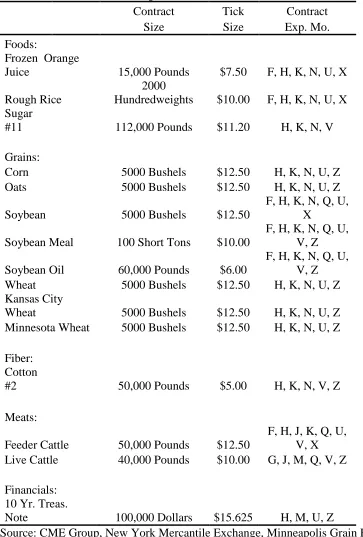
Data on futures contracts are from R & C Research, Inc. at Price-data.com. A listing of the differing commodity futures tested in the study is shown on Table 3. The listing is
not all inclusive as R & C Research only captures data in demand from consumers of their products. Futures such as dairy products are not listed because of a lack of available data. Others agricultural commodities such as poultry are not publicly traded on the
futures market. Table 3 also shows the symbol the futures exchanges use for each futures contract
Table 4 provides data on agricultural production in the United States as provided by the 2007 Census for Agriculture (USDA, 2007). Corn is the largest commodity by
46
commodity in terms of farmland used for production at 36.2%. Crops and livestock are very similar in total agricultural sales at 48.3 and 51.7% respectfully. As for agricultural
farmland needed for production, crops are grown on 44.7% as compared to livestock grazing on 49.0% of the land. The census data implies the futures contracts provided on
Table 3 appear to be sufficient and comprehensive enough to develop a representative sample for the current study. I include futures contracts in my model that are the leading crops produced in each specific region.2 Four to five differing crops are tested in each
region.
Agricultural commodity futures have differing contract specifications. Table 5 provides a listing of specifications for each commodity in the study. Each of the futures contracts has differing contract sizes and tick sizes. Tick sizes are the minimum fluctuation of the
price for a given futures contract and all of the commodities are $12.50 or less. The agricultural commodities are measured in pounds or bushels, with soybean meal and
rough rice being the exceptions as they are measured in short tons and hundredweights. Each of the futures contracts has daily price limits at varying rates. These daily limits are caused by commodity price volatility and the chance of catastrophic losses. Daily limits
may freeze prices, but do not freeze trading on the futures contracts. Most are variable and are not shown in Table 5 for the sake of brevity.3 Settlement procedures for
2
Seehttp://www.ers.usda.gov/Briefing/,
http://commodities.about.com/od/gettingstarted/a/profiles.htm,
http://www1.agric.gov.ab.ca/$department/deptdocs.nsf/all/sis5219, and http://www.epa.gov/oecaagct/ag101/cropmajor.html
3
47
agricultural commodity futures contracts are characterized by physical delivery of the goods, although many contracts settle before expiration. Most agricultural commodity
futures last trade date is the business day prior to the 15th day of the expiration month and delivery dates are commonly in the week following the last trading day of that same
month. Futures contracts expire in different months and very few agricultural futures contracts expire in all 12 months.
Table 5 shows the varying expiration months for each of the futures contracts. A limitation of the study is that expiration dates are not always on the 1st of each quarter
(January, April, July, and October). I interpolate the prices of the contracts that bracket the beginning of each quarter to match the data points and provide four points per year. Further, because of weekends and holidays, futures prices do not always occur on the 1st
day of the month, therefore I use the end of day trading price closest to that particular day.
Interest Rate Futures
Interest rate futures prices are taken from R & C Research, Inc. similar to agricultural
commodity futures. The 10-year treasury-note is used as a proxy for applicable interest rates in the study. Its ticker symbol is shown on panel A of Table 3. Buying an interest
rate futures contract allows a borrower to lock an anticipated interest rate in the present, while the underlying interest rate changes with the market. The rate being represented by the futures contract is an investment rate, not a borrowing rate of interest. The 10-year