www.hydrol-earth-syst-sci.net/18/1679/2014/ doi:10.5194/hess-18-1679-2014
© Author(s) 2014. CC Attribution 3.0 License.
Hydrology and
Earth System
Sciences
Predicting streamflows in snowmelt-driven watersheds using the
flow duration curve method
D. Kim and J. Kaluarachchi
College of Engineering, Utah State University, Logan, UT 84322-4100, USA
Correspondence to: D. Kim ([email protected])
Received: 5 June 2013 – Published in Hydrol. Earth Syst. Sci. Discuss.: 18 July 2013 Revised: 17 March 2014 – Accepted: 18 March 2014 – Published: 9 May 2014
Abstract. Predicting streamflows in snow-fed watersheds in the Western United States is important for water alloca-tion. Since many of these watersheds are heavily regulated through canal networks and reservoirs, predicting expected natural flows and therefore water availability under limited data is always a challenge. This study investigates the appli-cability of the flow duration curve (FDC) method for pre-dicting natural flows in gauged and regulated snow-fed wa-tersheds. Point snow observations, air temperature, precipi-tation, and snow water equivalent were used to simulate the snowmelt process with the SNOW-17 model, and extended to streamflow simulation using the FDC method with a mod-ified current precipitation index. For regulated watersheds, a parametric regional FDC method was applied to recon-struct natural flow. For comparison, a simplified tank model was used considering both lumped and semi-distributed ap-proaches. The proximity regionalization method was used to simulate streamflows in the regulated watersheds with the tank model. The results showed that the FDC method is capa-ble of producing satisfactory natural flow estimates in gauged watersheds when high correlation exists between current pre-cipitation index and streamflow. For regulated watersheds, the regional FDC method produced acceptable river diver-sion estimates, but it seemed to have more uncertainty due to less robustness of the FDC method. In spite of its simplicity, the FDC method is a practical approach with less computa-tional burden for studies with minimal data availability.
1 Introduction
Snow accounts for a significant portion of precipitation in the mountainous Western United States and snowmelt plays an important role in forecasting streamflow (Serreze et al., 1999). Extreme amounts of snowfall can result in a flood in the melting season, and sometimes snow accumulation alleviates drought by natural redistribution of precipitation in a high water-demand period. In such regions, snowmelt controls the hydrologic processes and water relevant activi-ties such as irrigation. Therefore, the reliable prediction of snowmelt is crucial for water resources planning and man-agement (He et al., 2011; Mizukami et al., 2011; Singh and Singh, 2001).
Conventionally, conceptual snowmelt models developed by combining rainfall–runoff models with temperature index models using a parameterized melting factor (e.g., Anderson, 2006; Albert and Krajeski, 1998; Neitsch et al., 2001), have been used to predict daily streamflows in snow-fed water-sheds. Conceptual modeling is an attractive solution to daily streamflow simulation not only for rainfall-fed but also for snow-fed watersheds due to its flexibility and applicability (Uhlenbrook et al., 1999; Smakhtin, 1999). Examples in-clude models such as SSARR (Cundy and Brooks, 1981), PRMS (Leavesley et al., 1983), NWSRFS (Larson, 2002), UBC (Quick and Pipes, 1976), CEQUEAU (Morin, 2002), HBV (Bergström, 1976), SRM (Martinec, 1975), and TANK (Sugawara, 1995), among others.
2006). Hence, the parameters of conceptual models are usu-ally identified by streamflow observations with calibration techniques such as the shuffled complex evolution or genetic algorithm. In truth, calibration is the major part of concep-tual modeling, and it is still typically labor-consuming; how-ever, computational efficiency has improved with advances in computer technology. In spite of the effort involved, un-certainty in conceptual models is always an important issue (Kuczera and Parent, 1998; Uhlenbrook et al., 1999; Panday et al., 2013). Furthermore, the parameter set calibrated by streamflow observations is usually not unique because there can be other sets of parameters providing similar model per-formance (Beven, 1993; Seibert, 1997; Oudin et al., 2006; Perrin et al., 2007). Particularly in snowmelt runoff model-ing, calibration can produce less uniqueness, less robustness, and more uncertainty than rainfall–runoff modeling because additional inputs (e.g., air temperature) and parameters (e.g., melting factor) are required to define the snowmelt process.
As an alternate approach, linking point snow observations to streamflow can be a pragmatic option. A common statisti-cal approach for simple generation of daily streamflow is the flow duration curve (FDC) method. A FDC gives a summary of streamflow variation and represents the relationship be-tween streamflow and its exceedance probability (Vogel and Fennessey, 1994). For streamflow generation, one or multi-ple sets of donor variables are transferred to a target station by corresponding exceedance probability of the donor sets with that of the target. A number of variations of the FDC method have been used for the generation of daily streamflow data. Hughes and Smakhtin (1996), for instance, suggested a FDC method with a nonlinear spatial interpolation method to extend observed flow data. Smakhtin and Masse (2000) de-veloped a variation of the FDC method to generate stream-flow using rainfall observations as the donor variable instead of streamflow data. Recently, the FDC was used not only for generating streamflow directly, but also for calibrating conceptual models (Westerberg et al., 2011). Westerberg et al. (2011) used the FDC as a performance measure to cir-cumvent uncertainty in discharge data and other drawbacks in model calibration with traditional methods. Despite the numerous applications with the FDC, there is still no good approach using the FDC method to generate daily stream-flow from point snow observations. Given the simplicity of the FDC method, a suitable approach using the FDC method to predict snowmelt-driven runoff using point snow observa-tions could be practical and cost efficient due to the reduced computational effort.
If the target station is ungauged, a regional FDC can es-timate the FDC of the target station. The regional FDC is generally developed using the relationships between selected percentile flows in gauged FDCs and climatic or physical properties of the watersheds. Thus, the regional FDC esti-mates the unknown FDC of an ungauged watershed only with its physical properties. Many regional FDC methods have been proposed for generating streamflows in ungauged
wa-tersheds. Shu and Ouarda (2012) categorized the regional FDC methods as a statistical approach (e.g., Singh et al., 2001; Claps et al., 2005), a parametric approach (e.g., Yu et al., 2002; Mohamoud, 2008), and a graphical approach (e.g., Smakhtin et al., 1997).
The regional FDC can be used not only for generating streamflows in ungauged watersheds, but also for recon-structing natural flows of watersheds regulated by reser-voir operations, river diversions and other human activities. Smakhtin (1999), for example, evaluated the impact of reser-voir operations by comparing between regulated outflows from a reservoir and natural flow estimated by a regional FDC. In the Western United States, the prior appropriation doctrine, the water right of “first in time, first in right,” has produced many river basins with impaired streamflows. These impairments are particularly significant in watersheds with high aridity, low precipitation, and relatively large wa-ter demands. The regional FDC method can represent flow impairments by reconstructing natural flows using minimal data. The reconstruction of natural flow provides additional information to water managers for efficient water alloca-tion during the high-demand periods. The volume difference between reconstructed natural flows and impaired stream-flow observations can simply indicate the combined effects of reservoir operations, river diversions, and other human-driven activities. Thus, the effect of regulation in a watershed can be approximately evaluated from this comparison.
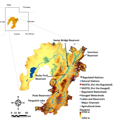
Fig. 1. Physical layout of the Sevier River basin, Utah.
2 Description of the study area and data
The study area is the Sevier River basin, located in South Central Utah, and the details are given Fig. 1. The Sevier River basin is a semi-arid basin with relatively high ET (evapotranspiration). The watersheds in or adjacent to the Sevier River basin are dominantly fed by snowmelt from the high-elevation region. Particularly, the Sevier River is signifi-cantly regulated by diversions and reservoir operations along the major channel for agricultural water use. Hence, a real-time streamflow monitoring system along the main channel is operated by the Sevier River Water Users Association, but it is difficult to estimate the natural discharge from the regu-lated watersheds using this monitoring system.
This study used the US Geological Survey (USGS) streamflow stations for the FDC method and conceptual modeling. Because only five watersheds in the Sevier River basin have natural streamflow observations, eight adjacent watersheds were included as well for generating streamflows in gauged watersheds. In addition, two USGS stations in the main Sevier River with significant impairments were selected for reconstructing natural flows using the regionalization methods. These two stations were assumed as ungauged wa-tersheds although these have continuous daily observations. Hence, “gauged” watersheds in this study refer to watersheds with natural flow observations only, while “regulated” water-sheds indicate waterwater-sheds with impaired flows and therefore these watersheds are treated as ungauged watersheds.
Precipitation, maximum and minimum air temperature, and snow water equivalent (SWE) data from the SNOTEL stations operated by US Department of Agriculture (USDA) were used as inputs to the FDC method and conceptual mod-eling. The details of the USGS stations and corresponding SNOTEL stations are given in Table 1 with corresponding data periods and watershed areas. Additionally, the records of canal diversions from the Utah Division of Water Rights were used to compare streamflows simulated by regionaliza-tion with actual river diversions. For the conceptual model-ing, point SNOTEL data were adjusted to spatially averaged inputs using data from the PRISM database (PRISM Climate Group, 2012). The procedure included a comparison between a pixel located in a SNOTEL station and the areal average of pixels in a watershed or an elevation zone using 30 arcsec an-nual normals from 1981 to 2010. The ratio of the average of pixels to the pixel at a SNOTEL station was multiplied by the point precipitation at the SNOTEL station, while the differ-ence between these was added to the point temperature. For the regional FDC, the SNOTEL data adjusted by PRISM data were also used for calculating climatic variables. The USGS National Elevation Dataset (2012) and US General Soil Map served by USDA (2013) were used to obtain geomorphologic and soil properties of the watersheds.
3 Methodology
3.1 SNOW-17 snowmelt model
Table 1. Details of gauged watersheds and corresponding USGS and SNOTEL stations.
# USGS station Gauged watershed Area (km2) SNOTEL station Data period (water year
a)
Calibration Validation 1 10173450 Mammoth Creek 271.9 Castle Valley 2001–2006 2007–2011 2 10174500 Sevier River at Hatch 880.6 Midway Valley 2001–2006 2007–2011 3 10194200 Clear Creek 424.8 Kimberly Mine 2001–2006 2007–2011 4 10205030 Salina Creek 134.2 Pickle KEG 2001–2006 2007–2011 5 10215900 Manti Creek 68.4 Seeley Creek 2001–2006 2007–2011 6 10242000 Coal Creek 209.5 Webster Flat 2001–2006 2007–2011 7 10234500 Beaver River 235.7 Merchant Valley 2001–2006 2007–2011 8 10172700 Vernon Creek 64.7 Vernon Creek 2001–2006 2007–2011 9 10146000 Salt Creek 247.6 Payson R.S. 2001–2006 2007–2011 10 09310500 Fish Creek 155.7 Mammoth-Cottonwood 2001–2006 2007–2011 11 09326500 Ferron Creek 357.4 Buck Flat 2001–2006 2007–2011 12 09330500 Muddy Creek 271.9 Dill’s Camp 2001–2006 2007–2011 13 09329050 Seven Mile Creek 62.2 Black Flat-U.M. CK 1992–1998 2008–2011
aWater year (WY): 1 year from 1 October in the previous year to 3 September in the current year.
calibration. Parameters were optimized using the genetic al-gorithm in the Matlab environment. The NSE for snowmelt modeling (NSESWE)is defined as
NSESWE=1−
PT
t=1
n
QSWE(t )− ˆQSWE(t )
o2
PT
t=1
QSWE(t )−QSWE
2 , (1)
whereQSWE(t ) andQˆSWE(t ) are observed and simulated SWEs (mm) at timet, respectively,QSWE is the mean ob-served SWE (mm), andT is the number of observations. 3.2 Modified FDC method with precipitation index
The FDC method is a non-parametric probability density function representing the relationship between magnitude of streamflow and its exceedance probability. The FDC method is typically used to generate daily streamflow at a station from highly correlating donor streamflow data sets with a tar-get station. A drawback of this approach is that streamflow generation is dependent on the availability of donor data sets. Hence, in a region with a low density of stream gauging sta-tions, the FDC method may face the difficulty of not having adequate donor streamflow data.
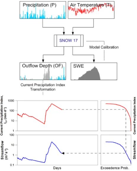
Smakhtin and Masse (2000) developed a modified FDC method with a precipitation index to overcome the limited availability of donor variable sets. Their method included transforming the time series of precipitation into an index having similar properties to streamflow data. The transfor-mation was to avoid zero values in precipitation data caused by the intermittency of precipitation events, which there-fore produce a different shape of duration curve from a typ-ical FDC. The duration curve of transformed precipitation could indicate the exceedance probability at the outlet, which determines the magnitude of streamflow.
This study modified the original concept as follows. First, the outflow depth simulated by SNOW-17 was used for con-structing the FDC instead of precipitation data to represent the snowmelt process. Second, a constant recession coeffi-cient was applied for the calculation of precipitation index of Smakhtin and Masse (2000), but different coefficients were used to represent the different hydrologic responses of rain-fall and snowmelt to streamflow. The modified approach is given below.
The current precipitation index at timet,ICP(t )in mm d−1 was defined in the original work as
ICP(t )=k·ICP(t−1)·1t+P (t ), (2) wherekis the recession coefficient (d−1),P (t )is daily pre-cipitation at timet(mm d−1), and1tis the time interval (d). Recession coefficient,k, represents the similar concept to the baseflow recession coefficient and needs to be determined by observed streamflow. According to previous studies, k
varies from 0.85 to 0.98 d−1(Linsley et al., 1982; Fedora and Beschta, 1989). In addition, the initial value ofICPcan be as-sumed as the long-term mean daily precipitation because of the fast convergence of calculations (Smakhtin and Masse, 2000).
Fig. 2. Details of the proposed modeling approach with the FDC
method and the SNOW-17 model.
ICP(t )=ICS(t )+ICR(t )
ICS(t )=kS·ICS(t−1)·1t+S(t ) (3)
ICR(t )=kR·ICR(t−1)·1t+R(t ),
whereICS(t )is the current snowmelt index (mm) at timet,
S(t )is the snowmelt depth (mm) at timet,ICR(t )is the cur-rent rainfall index (mm) at timet,R(t )is the rainfall depth (mm) at timet,kSandkRare recession coefficients (d−1)for snowmelt and rainfall, respectively. Generally,kS is greater thankRbecause snowmelt runoff varies more smoothly with time than quick flow caused by rain storms. In this study,
kSandkRwere selected by values showing maximum corre-lation betweenICP and observed streamflow data. Figure 2 shows the proposed FDC method used in this work.
[image:5.595.313.547.62.197.2]The selection of a snow observation station when multiple stations are present in a watershed was based on high corre-lation between calculatedICPand observed streamflow. Al-though Smaktin and Masse (2000) commented that the effect of weights in the case of multiple stations was not a signif-icant factor in their original FDC method with the precipi-tation index, a high correlation betweenICPand streamflow supports better performance in the generation of streamflow because of the significant climatic variation of snow-fed wa-tersheds located in high-elevation regions.
Fig. 3. Details of the proposed approach with the tank model and
SNOW-17.
3.3 Simplified tank model
This study used the simplified tank model proposed by Cooper et al. (2007) to compare the performance under the conditions of similar and limited data availability. The sim-plified tank model reduced the number of parameters of the original tank model (Sugawara, 1995) to help minimize over-parameterization when the tank model was combined with the snowmelt model. This simplified tank model shown in Fig. 3a has two vertical layers with the primary soil mois-ture layer in the upper tank. This study did not consider the secondary soil moisture layer in the simplified tank model because it was not sensitive to runoff simulations (Cooper et al., 2007). Evapotranspiration (ET) in the tank model was independently estimated using the modified complementary method proposed by Anayah (2012). The combined model has 12 parameters (5 for snowmelt, 7 for runoff). The struc-ture of the tank model is adequately flexible to be calibrated by streamflow observations. It has more parameters than the Snowmelt Runoff Model with eight parameters (Martinec et al., 2008).
The model produces several modes of response repre-senting the different conditions that may prevail in a wa-tershed. The upper tank has a non-linear response in the rainfall–runoff process because of its multiple horizontal out-lets, whereas the lower tank has a linear response. There are three thresholds to determine the four modes of hydro-logic response, which areHS,H1, andH2.HSrepresents the soil moisture-holding capacity (mm). H1 andH2 represent the lower and upper thresholds for generating direct runoff (mm). The detailed procedure for calculating streamflow is available from Cooper et al. (2007).
tanks for the upper layer to accommodate climatic variation due to elevation (Fig. 3b). All of the upper tanks in both ap-proaches were assumed to have same parameters for both snowmelt and runoff modeling. For the semi-distributed tank model, a watershed was divided into five zones with the aid of the area–elevation relationship. Inputs for each zone were individually computed from the corresponding SNOTEL sta-tion and PRISM data as explained earlier.
The parameters were optimized using the genetic algo-rithm in Matlab for both the lumped and the semi-distributed tank models with the objective function of minimizing the sum of weighted squared residuals shown as below.
Minimize T X
t=1
w(t )·nQ(t )− ˆQ(t )o
2
, (4)
where w(t ) is weight (unitless) varying with magnitude of runoff data, Q(t ) andQ(t )ˆ are observed and simulated streamflows (m3s−1), respectively, andT is the number of observations. The weights can be determined empirically with observed data for equalizing residuals in low flows with those in high flows. The weights used in previous studies (e.g., Kim and Kaluarachchi, 2008, 2009) ranged from 4 to 10. The average streamflows of gauged watersheds in the high flow season (April to June) were about 2 to 10 times (with median of 5.17) those in the low flow season (March to June). Hence, this study used a weight of 5 for the low runoff season and 1 for the high runoff season. Although Cooper et al. (2007) proposed two constraints to calibrate the tank model parameters with wide ranges, incorporating SNOW-17 into the tank model made it difficult to apply the constraints to the combined model. Hence, in the optimization with ge-netic algorithm, the ranges of parameters were identified us-ing Monte Carlo simulations with uniform distributions. One of the best 100 parameter sets obtained by sorting the values of the objective function was selected to set the parameter ranges for genetic algorithm.
3.4 Regionalization
This study applied regionalization to simulate natural stream-flows in regulated watersheds with impaired observations. A parametric approach was selected for constructing the re-gional FDC. The model proposed by Shu and Ouarda (2012) was used and given as
QP=aV1bV2cV3d. . . , (5) where QP is percentile flows, V1, V2, V3,. . . are selected physical or climatic descriptors, b, c, d,. . . are model pa-rameters, andais the error term. Logarithmic transformation of Eq. (5) can help solve the model through linear regres-sion. By step-wise regression, independent variables can be selected.
[image:6.595.308.547.64.182.2]Meanwhile, a proximity-based regionalization method was used for the tank model. In the case of conceptual mod-eling, regionalization of parameters for ungauged watersheds
Fig. 4. Results from SNOW-17 at SNOTEL stations: (a) Castle
Val-ley, (b) Pickle KEG, and (c) Vernon Creek.
were categorized by three approaches (Peel and Blöschl, 2011): (a) regression analysis between individual parame-ters and waparame-tershed properties (e.g., Kim and Kaluarachchi, 2008; Gibbs et al., 2012); (b) parameter transfer based on spatial proximity (e.g., Vandewiele et al., 1991; Oudin et al., 2008); and (c) physical similarity (e.g., McIntyre et al., 2005; Oudin et al., 2008, 2010). Even if the performance of these three approaches was dependent on climatic conditions, per-formance and complexity of the model, and other factors, several studies concluded that the spatial proximity method was attractive due to its better performance and simplicity (Oudin et al., 2008; Parajka et al., 2013). Hence, this study used the proximity-based regionalization for regulated water-sheds. Parameter sets were transferred from multiple gauged watersheds for better precision, and the average of stream-flows simulated by the parameter sets was taken as the natural flow estimates for the regulated watersheds.
4 Results
4.1 SNOW-17 modeling
SNOW-17 was calibrated and verified by SWE observations at SNOTEL stations. Figure 4 shows the results of SNOW-17 modeling where the comparison between simulated and ob-served SWE is excellent. The average NSE values between simulated and observed SWE for calibration and validation were 0.942 (a range of 0.867 to 0.984) and 0.933 (a range of 0.793 to 0.967), respectively. The loss of NSE from calibra-tion to validacalibra-tion was not significant and therefore the model was unlikely to be over-parameterized. Also, the simple ob-jective function of maximizing NSE (equivalent to minimiz-ing the sum of squared residuals) seems to provide adequate performance as long as accumulated precipitation shows a consistent trend with observed SWE in the snow accumu-lation period. Simultaneous monitoring of precipitation and SWE at the same location may provide quality inputs to SNOW-17 modeling.
(Anderson, 1976). In other words, good calibration by SWE observations does not necessarily guarantee accurate simula-tion of outflow depth. The loss of SWE by winds or subli-mation, for instance, is not contributing to the melting depth while some SWE reduction is observed. Thus, in a region with high possibility of such errors, caution is required to link point snowmelt observations to streamflow.
4.2 Streamflow generation in gauged watersheds
The time series of outflow depth from SNOW-17 was used to calculateICP. Since the rationale behind the FDC method is that exceedance probability ofICPis same as that of stream-flow, the data periods of both point snow observations and streamflow data should be same. In fact,ICP calculation is mathematically equivalent to the computation of storage in a single linear reservoir such as the lower tank in the tank model. Hence, the hydrological meaning ofICPis liquid wa-ter availability in a wawa-tershed with the assumption of a single linear reservoir. Through theICPcomputation, the intermit-tent time series of outflow depth was transformed to a smooth time series.
The computed recession coefficients of snowmelt varied from 0.97 to 0.98 d−1, while the range for rainfall was 0.85 to 0.86 d−1. These results demonstrate that snowmelt runoff was slowly changing during the year, unlike rainfall runoff that showed a relatively large fluctuation due to the inter-mittent storm events. In the study area, snowmelt runoff ac-counted for a large portion of streamflow and therefore the recession coefficient of snowmelt played a major role in the high correlation between ICP and streamflow. However, if there was noticeable contribution of rainfall runoff to stream-flow observations, then the recession coefficient of rainfall would be more important and sensitive. Particularly, rainfall runoff can be crucial in the non-melting season, and there-fore, the separation of recession coefficients is necessary for high correlation betweenICPand streamflow.
When calibrating the lumped and semi-distributed tank models, Monte Carlo method was used to identify the pa-rameter ranges of the tank model for optimization with ge-netic algorithm as commented earlier. The random simula-tions were to avoid local parameter sets providing unrealis-tic or poor streamflow simulation when using geneunrealis-tic algo-rithm with wide parameter ranges. To decide on the required number of simulations, the Clear Creek watershed was se-lected and tested among the given gauged watersheds. By increasing the number of simulations from 1000 to 20 000, it found that 20 000 simulations provided the efficient num-ber of simulations with the initial parameter ranges. From the best 100 parameter sets of the 20 000 simulations, a pa-rameter set with an acceptable NSE and a low reduction of NSE between calibration and validation was chosen. For op-timization with genetic algorithm, the parameter ranges were rescaled with the ranges of approximately 50 to 200 % of each parameter of the chosen set. With the rescaled
param-Fig. 5. Simulated streamflows with the FDC and the tank model: (a) Ferron Creek, (b) Sevier River at Hatch, (c) Vernon Creek, and (d) Fish Creek.
eter ranges, the genetic algorithm produced the optimal pa-rameter set. It was later found that the optimal papa-rameter set showed better performance than the best 100 parameter sets of the 20 000 simulations for all gauged watersheds. From this observation, the optimal parameter set was assumed as the calibrated parameter set.
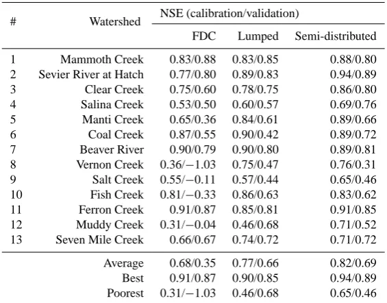
[image:7.595.310.545.63.448.2]Table 2. Performance comparison between the FDC method and the tank models.
# Watershed NSE (calibration/validation)
FDC Lumped Semi-distributed 1 Mammoth Creek 0.83/0.88 0.83/0.85 0.88/0.80 2 Sevier River at Hatch 0.77/0.80 0.89/0.83 0.94/0.89 3 Clear Creek 0.75/0.60 0.78/0.75 0.86/0.80 4 Salina Creek 0.53/0.50 0.60/0.57 0.69/0.76 5 Manti Creek 0.65/0.36 0.84/0.61 0.89/0.66 6 Coal Creek 0.87/0.55 0.90/0.42 0.89/0.72 7 Beaver River 0.90/0.79 0.90/0.80 0.89/0.81 8 Vernon Creek 0.36/−1.03 0.75/0.47 0.76/0.31 9 Salt Creek 0.55/−0.11 0.57/0.44 0.65/0.46 10 Fish Creek 0.81/−0.33 0.86/0.63 0.83/0.62 11 Ferron Creek 0.91/0.87 0.85/0.81 0.91/0.85 12 Muddy Creek 0.31/−0.04 0.46/0.68 0.71/0.52 13 Seven Mile Creek 0.66/0.67 0.74/0.72 0.71/0.72 Average 0.68/0.35 0.77/0.66 0.82/0.69 Best 0.91/0.87 0.90/0.85 0.94/0.89 Poorest 0.31/−1.03 0.46/0.68 0.65/0.46
the on and off snow cover of the lumped tank model. How-ever, the FDC method could be competitive when point snow observations are highly correlated with streamflow. Ferron Creek, Beaver River, and Mammoth Creek, which had fairly high correlation betweenICP and streamflow data, showed good performance in streamflow prediction. Even the semi-distributed tank model did not show better results than the FDC method for Ferron Creek and Beaver River.
Typically, watersheds showing good performance with the FDC method have good performance with the lumped and semi-distributed tank models too. Since both methods used linear reservoir coefficients for simulating streamflow, they performed well in watersheds with linear behavior and such watersheds were likely to have relatively homogenous cli-matic conditions. In addition, the FDC method showed the highest performance reduction from calibration to validation among the three methods. This may be due to the unstable correlation betweenICP and streamflow and the uncertainty of the FDCs.
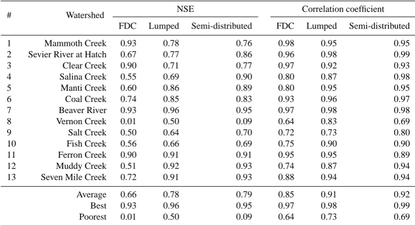
Figure 6 shows a comparison between field discharge mea-surements and simulated streamflows in the calibration pe-riod. In order to avoid potential errors in streamflow obser-vations converted from water stage, streamflow simulations by three methods were directly evaluated by field measure-ments. Table 3 summarizes the NSE and correlation coef-ficient values between field measurements and three simu-lations. Streamflow values for this evaluation were normal-ized by watershed area to remove the influence of water-shed scale. On average, the performance trend from the poor-est to the bpoor-est watersheds was similar to the calibrations with the continuous streamflow data in terms of NSE. How-ever, Vernon Creek and Salt Creek experienced a large
re-Fig. 6. Comparison between field discharge measurements and
streamflow simulations (discharges are normalized by watershed area).
[image:8.595.313.542.328.473.2]Table 3. NSE and correlation coefficient between field measurements and the three model simulations.
# Watershed NSE Correlation coefficient FDC Lumped Semi-distributed FDC Lumped Semi-distributed 1 Mammoth Creek 0.93 0.78 0.76 0.98 0.95 0.95 2 Sevier River at Hatch 0.67 0.77 0.86 0.96 0.98 0.99 3 Clear Creek 0.90 0.71 0.77 0.97 0.92 0.93 4 Salina Creek 0.55 0.69 0.90 0.80 0.87 0.98 5 Manti Creek 0.60 0.86 0.89 0.80 0.95 0.95 6 Coal Creek 0.74 0.85 0.83 0.93 0.96 0.97 7 Beaver River 0.93 0.96 0.95 0.97 0.98 0.98 8 Vernon Creek 0.01 0.50 0.09 0.64 0.83 0.69 9 Salt Creek 0.50 0.64 0.70 0.72 0.73 0.80 10 Fish Creek 0.56 0.66 0.69 0.75 0.90 0.90 11 Ferron Creek 0.90 0.91 0.91 0.95 0.95 0.89 12 Muddy Creek 0.51 0.92 0.93 0.74 0.87 0.94 13 Seven Mile Creek 0.72 0.91 0.93 0.88 0.94 0.94 Average 0.66 0.78 0.79 0.85 0.91 0.92 Best 0.93 0.96 0.95 0.97 0.98 0.99 Poorest 0.01 0.50 0.09 0.64 0.73 0.69
4.3 Regional FDC for regulated watersheds
The FDC method and the tank model were upscaled to wa-tersheds affected by river diversions and reservoir operations to predict the natural flows at impaired streamflow stations. As mentioned earlier, regionalization was used for upscal-ing of regulated watersheds. The regulated station near the Piute Reservoir (Fig. 1) is Seveir River near Kingston, and the other near the Sevier Bridge Reservoir is Sevier River below San Pitch River near Gunnison (hereafter Sevier River near Gunnison).Water use in agricultural areas through river diversions significantly affect streamflow observations in the two stations. Streamflow observations at Sevier River near Kingston only include river diversions while the diversions and reservoir operations are included in streamflow obser-vations at Sevier River near Gunnison. The two watersheds were divided into several sub-watersheds because these were too large to fall within the areas of gauged watersheds used for developing the regional FDCs. Hence, the sum of stream-flows of each sub-watershed simulated by regionalization was the volume of natural flow at each target station.
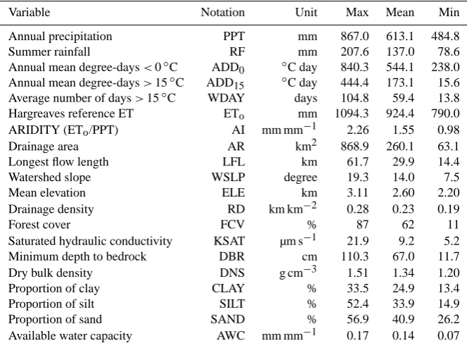
Climatic, geomorphologic, land cover and soil properties of the gauged watersheds were used to identify independent variables in determining the percentile flows of the paramet-ric regional FDC. The candidate properties are listed in Ta-ble 4. The step-wise regression was implemented for each percentile flow in the Matlab environment. The variable with the largest significance among the candidates was taken as an independent variable for the first step. Then, other variables were added step by step based on thepvalue of F statistics. The selected variables for each percentile flow and the statis-tics of the regression analysis are given in Table 5. Overall, the regional FDC reproduced minimum, average, and
stan-dard deviation well, but underestimated the maximum of per-centile flows. This means the regional FDC may underesti-mate percentile flows of large watersheds; therefore it is not recommended to use the regional FDC for an ungauged wa-tershed with an area larger than the largest wawa-tershed of the regression model.
As expected, watershed area was included in every per-centile flow as an independent variable. Watershed area was positively related to percentile flows, and its multipliers ranged from 0.5 to 1.0. The multiplier had an increasing ten-dency as percentile increases. The routing effect on high flow (low percentile) may cause less proportionality to watershed area than low flow (high percentile).
Also, mean elevation was selected as another crucial in-dependent variable. The multiplier of elevation varied from 2.2 to 3.7. Elevation was considered to be a geomorphologic property, but it represented the climatic variation of the wa-tersheds because every climatic candidate had high correla-tion with elevacorrela-tion. It is a natural observacorrela-tion because more precipitation and lower air temperature are expected in the higher elevations.
Table 4. Candidate variables for the multiple linear regression analysis.
Variable Notation Unit Max Mean Min Annual precipitation PPT mm 867.0 613.1 484.8 Summer rainfall RF mm 207.6 137.0 78.6 Annual mean degree-days<0◦C ADD0 ◦C day 840.3 544.1 238.0 Annual mean degree-days>15◦C ADD15 ◦C day 444.4 173.1 15.6
Average number of days>15◦C WDAY days 104.8 59.4 13.8 Hargreaves reference ET ETo mm 1094.3 924.4 790.0
ARIDITY (ETo/PPT) AI mm mm−1 2.26 1.55 0.98
Drainage area AR km2 868.9 260.1 63.1 Longest flow length LFL km 61.7 29.9 14.4 Watershed slope WSLP degree 19.3 14.0 7.5 Mean elevation ELE km 3.11 2.60 2.20 Drainage density RD km km−2 0.28 0.23 0.19 Forest cover FCV % 87 62 11 Saturated hydraulic conductivity KSAT µm s−1 21.9 9.2 5.2 Minimum depth to bedrock DBR cm 110.3 67.0 11.7 Dry bulk density DNS g cm−3 1.51 1.34 1.20 Proportion of clay CLAY % 33.5 24.9 13.4 Proportion of silt SILT % 52.4 33.9 14.9 Proportion of sand SAND % 56.9 40.9 26.2 Available water capacity AWC mm mm−1 0.17 0.14 0.07
Table 5. Selected variables and statistics of the regional FDC method.
Percentile flow Selected variables R2 Observed Estimated
Max Mean Min Stda Max Mean Min Std
Q0.1 AR, ELE, CLAY 0.86 48.65 16.96 1.04 13.10 40.59 16.12 1.16 11.42
Q1 AR, ELE, CLAY 0.94 37.87 11.54 0.59 8.99 27.58 11.28 0.63 8.37
Q5 AR, ELE, CLAY 0.93 12.94 4.56 0.24 3.48 10.27 4.46 0.27 3.19
Q10 AR, ELE, CLAY 0.93 6.31 2.39 0.16 1.74 5.58 2.34 0.16 1.63
Q20 AR, ELE, CLAY 0.92 3.40 1.10 0.13 0.86 2.87 1.05 0.12 0.73
Q30 AR, ELE, DNS 0.93 2.72 0.74 0.09 0.67 2.04 0.70 0.09 0.51
Q40 AR, ELE, DNS 0.94 2.01 0.85 0.08 0.49 1.39 0.50 0.08 0.35
Q50 AR, ELE, KSAT 0.95 1.56 0.42 0.07 0.37 1.04 0.40 0.06 0.25
Q60 AR, ELE, KSAT 0.92 1.39 0.35 0.07 0.33 0.83 0.33 0.06 0.20
Q70 AR, ELE, KSAT 0.91 1.22 0.31 0.06 0.29 0.83 0.30 0.05 0.21
Q80 AR, ELE, KSAT 0.86 1.10 0.27 0.05 0.27 0.82 0.27 0.05 0.21
Q90 AR, RD, ELE, KSAT 0.96 1.05 0.24 0.05 0.26 0.82 0.23 0.04 0.21
Q95 AR, RD, ELE, KSAT 0.95 0.96 0.21 0.03 0.25 0.73 0.20 0.04 0.19
Q99 AR, RD, ELE, KSAT 0.97 0.88 0.18 0.02 0.23 0.65 0.17 0.02 0.17
Q99.9 AR, RD, ELE, KSAT 0.82 0.83 0.15 0.01 0.22 0.48 0.13 0.02 0.14 aStd: Standard deviation.
was included as an additional significant variable for low flows with negative relationships. The negative relationship is probably because the higher drainage density means more distribution of streamflow in a watershed.
When using the regional FDC approach, ICP was not necessarily used as the only donor variable to transfer ex-ceedance probability to the target stations. In fact, the best donor variable is a data set that can show the best correlation with gauged streamflow at the target station. However, it is
impossible to check the correlation between donor variables and ungauged streamflow. Thus, one or multiple donor vari-ables close to the target station have been typically used in the regional FDC approaches. Shu and Ouarda (2012) sug-gested using multiple donor variables to minimize the un-certainty of using a single donor variable. This study used two sets of neighboring streamflow observations as well as
[image:10.595.74.519.368.571.2]Fig. 7. Simulated streamflow in regulated watersheds: (a) Sevier
River near Kingston, and (b) Sevier River near Gunnison. FDC, Tank (L), and Tank (D) of the inside 1 : 1 plots are streamflows in m3s−1simulated by the FDC method, lumped tank, and semi-distributed tank models, respectively.
[image:11.595.51.286.64.189.2]for snowmelt and rainfall, respectively. As commented ear-lier, parameters of both lumped and semi-distributed tank models were transferred from nearby gauged watersheds for streamflow simulation at the target stations. The parameter sets of Mammoth Creek, Sevier River at Hatch, Coal Creek, and Beaver River were used for Sevier River near Kingston while Salina Creek, Manti Creek, Ferron Creek, and Seven-mile Creek were selected for Sevier River near Gunnison. Figure 7 shows the simulated streamflows by the regional FDC and the tank models with regionalized parameters at both target stations. In the case of Sevier River near Gunni-son, the outflow from the Rocky Ford Reservoir was sub-tracted from the observed streamflow to calculate the dis-charge produced by the watershed only. It could be easily recognized that these two watersheds were significantly reg-ulated based on the irregular shapes of hydrographs. At Se-vier River near Kingston, the regional FDC method estimated more volume of natural flow than the lumped and the dis-tributed tank models. On the other hand, water volume es-timated by the regional FDC was between the estimates of the lumped and semi-distributed models at Sevier River near Gunnison. Volume errors between the regional FDC method and the tank models varied from −17.1 to +21.8 %. The differences among the three methods were mainly in mid-dle to high flows rather than low flows. The correlation co-efficients between the simulations with the regional FDC and the lumped tank model were 0.94 and 0.70 at both sta-tions, respectively, while those between the regional FDC and the semi-distributed tank model were 0.92 and 0.90, re-spectively. The larger difference between the lumped and semi-distributed models at Sevier River near Gunnison may be due to the higher climatic variation of this watershed, making the lumped assumption inappropriate. This is evident from the greater difference of NSE between the lumped and semi-distributed models of gauged watersheds transferred to Sevier River near Gunnison.
Fig. 8. Model performance vs. correlation betweenICPand
stream-flow. Note correlation coefficient is calculated only when ex-ceedance probability is less than 0.2. For validation, only positive NSEs are plotted.
5 Discussion
5.1 FDC method for gauged watersheds
The basis of the FDC method is point snowmelt model-ing with SNOW-17. SNOW-17 performed well for the study area, but its parameter uncertainty could be a concern similar to conceptual runoff modeling. However, the five parameters used in SNOW-17 were small when compared to most clas-sical hydrologic models. Indeed, a simpler snowmelt model (e.g., DeWalle and Rango, 2008) or observed snowmelt depth (equivalent to a reduction in observed SWE) could be an al-ternative for SNOW-17, while not necessarily reducing the uncertainty.
The performance of the FDC method was affected by the correlation betweenICPand streamflow. Particularly, the cor-relation betweenICPand middle to high flow determined the performance. Figure 8 shows the relationship between the performance and the correlation coefficient betweenICPand streamflow with exceedance probability less than 0.2. Based on this knowledge, good performance (NSE>0.8) could be expected when the correlation coefficient is greater than 0.8. The greater NSE in the validation period of Mammoth Creek and Sevier River at Hatch (Table 2) than in the calibration pe-riod could be explained by the correlation coefficient. These two watersheds had greater correlation coefficients (about 0.04 differences for both watersheds) in the validation pe-riod. The stable FDCs found for both watersheds also sup-ported the better performance during validation.
the FDC method has a much wider range from the poorest to the best performing watersheds than the others. Indeed, more watersheds showed better NSE, as the inputs were more dis-tributed. This means that considering only point inputs with the FDC method could result in highly variable performance. Also, more distributed inputs would be better for more ro-bust performance, even in the case of a simple model. With the FDC method, its low input requirement and computa-tional burden has to be traded with some loss of robustness of performance.
In general, the FDC method had a poorer performance than the lumped and the semi-distributed tank models. One reason may be that the tank model was directly calibrated to streamflow observations, while the FDC method matched the magnitudes ofICPand streamflow based on an empirical probability density function. However, the main reason was that correlation betweenICPand streamflow could be lower significantly from one period to another. Fish Creek, for in-stance, experienced a reduced correlation coefficient (about 0.35) from calibration to validation. On the other hand, the lumped and semi-distributed models that considered spa-tial variations did not have such large reductions in NSE. It means a point snow observation might not represent the behavior of an entire watershed. Hence, the first task is to as-sess the applicability of the FDC method by evaluating the correlation betweenICPand streamflow.
There could be many reasons for the low correlation be-tweenICPand streamflow. For example, Vernon Creek and Muddy Creek showed poor performances with the FDC method, but the reasons were different. Vernon Creek is close to the Sevier Desert, which has extremely low excess pre-cipitation, unlike Muddy Creek. Thus, the consideration of other hydrological processes was necessary for Vernon Creek (ET in the lumped tank model) while the spatial variation of inputs is required for Muddy Creek. If ET is considered in the FDC method when computingICP, the FDC method may perform better than the proposed approach.
5.2 Regional FDC method for regulated watersheds
It is impossible to evaluate the correlation betweenICP and streamflow observation for regulated watersheds. With the low robustness of performance, usingICPas the only donor variable could result in a large bias in streamflow generation. Even in the case of transferring multipleICPvalues, the bias would not be small due to the performance variability of the FDC method. Thus, the use ofICPwas limited as one of the multiple donor variables. Neighboring streamflow observa-tions were also transferred in order to make up the drawback of ICP. Hence, the role of ICP for regulated (or ungauged) watersheds was to capture the hydrologic responses not in-cluded in the neighboring streamflow observations.
The simulated streamflows were higher than observed from April to October due to river diversions for agricul-ture at both regulated watersheds, except for year 2011 at
Sevier River near Gunnison. Sevier River near Gunnison is located below the intersection between the Sevier River and the San Pitch River, but it was difficult to know the stream-flow from the San Pitch River on a regular basis. Streamstream-flow in the San Pitch River was negligible in dry and normal years due to the high agricultural water demand in the San Pitch River basin, but it could not be neglected in a wet year such as 2011. Thus the observed streamflows at Sevier River near Gunnison were greater than the simulated natural flows in a wet year as shown in Fig. 7b.
Conceptually, when the simulated streamflow is greater than the observed flow, the difference indicates the volume of diversions. However, a similar difference could be as-sumed to represent the volume of return flow from the agri-cultural areas when the observation is greater than the sim-ulated value. As depicted in Fig. 7a, streamflow not de-caying from November to March (the period of no diver-sions) demonstrated that the return flows through infiltration affected streamflow continuously. Return flows may affect streamflow during the period of diversions, but it was dif-ficult to estimate the impact due to the complexity of com-bined flow. Simply, a positive difference between the simu-lated and observed flows in Fig. 7a indicated diversions in-cluding return flows, whereas a negative difference indicated return flow.
This study used observed diversions in the watersheds to validate the simulated natural streamflow. Most river diver-sions above Sevier River near Kingston were recorded for management purposes. Due to the high efficiency of water use in the agricultural area above this station, the effect of surface return flows may be small or negligible during the pe-riod of diversions. Even though the return flows through in-filtration may affect streamflow, it was relatively small when compared to the total diversions and streamflow during the period of diversions. If one assumes that there is no signifi-cant return flows during the diversion season, the difference between simulated and observed flows could be considered to be the volume of diversions.
Table 6 shows the sum of observed diversions in the main channel of the Sevier River above Sevier River near Kingston and the estimated volumes from the three methods. The ac-tual volume of diversions would be a little greater than the observed because some diversions might not be observed in spite of the large coverage of the diversion monitoring in the watershed. Hence, although Table 6 shows that the re-gional FDC method provided a larger natural flow than the others, the estimated volume of diversions by the regional FDC method could be considered a possible prediction.
Table 6. Estimated impairment and observed canal diversions at Sevier River near Kingston from April to September. The numbers within
parentheses are percent difference from the observed volume.
Year Estimated volume of diversion (×10
6m3)
Observed volume of FDC Lumped tank Semi-distributed tank diversion (×106m3)
2008 108 (+36 %) 69 (−13 %) 81 (+2 %) 79 2009 110 (+32 %) 61 (−25 %) 78 (−5 %) 82 2010 137 (+86 %) 95 (+29 %) 112 (+51 %) 74 2011 165 (+46 %) 132 (+19 %) 145 (+31 %) 111
semi-distributed model provides the most trustworthy results due to its better performance. Shu and Ouarda (2012) recom-mended at least four streamflow observations as donor vari-ables for good precision with the FDC methods. Thus, the re-gional FDC with two streamflows andICPin this study could add more uncertainty than a case with more donor variables. An important goal of this work in using the regional ap-proaches was to estimate the amount of water from stream-flow without actual diversion data. In most of these situa-tions data are limited, yet water managers require such in-formation to better manage water demands. The results of this analysis, especially from Table 6, shows the regional FDC method could produce acceptable estimates with less time and effort than conceptual modeling. There are several limitations in the regional FDC method. For every region-alization approach, including the regional FDC method, ad-equate streamflow observations are necessary to have good estimates. Parajka et al. (2013) commented that studies with more than 20 gauging stations produced better and stable performance with deterministic models. The regional FDC method is also sensitive to the number of gauging stations. Although the density of gauging stations was low in this study, gauged watersheds in the regional analysis should be adequate in terms of the watershed scale and climatic char-acteristics to minimize bias. As mentioned earlier, multiple donor variables can also minimize errors caused by bias of a single donor set.
6 Conclusions
In this study, a conceptual snowmelt model, SNOW-17, us-ing point snow observations, was extended usus-ing a modified FDC method to simulate streamflows in the semi-arid and mountainous Sevier River basin of Utah. The FDC method was later extended to simulate natural streamflows in regu-lated watersheds by incorporating a parametric regional FDC method. The FDC method could be a simple practical ap-proach for streamflow generation for watersheds with limited data. The FDC method was compared with the lumped and semi-distributed tank models under similar data availability to simulate streamflows and later extended via regionaliza-tion to estimate natural flows in regulated watersheds.
SWE observations as shown here. Other studies are neces-sary to determine the parameters of the snowmelt model for watersheds without SWE observations. Also, the difficulty of determining the recession coefficients forICPcalculation in ungauged watersheds is another remaining issue, since the typical values for gauged watersheds are assumed. In sum-mary, the FDC approach used here could produce practical values of expected streamflows from point observations for watersheds with limited data.
Acknowledgements. This research was funded by the Utah Water
Research Laboratory in Logan, UT. The authors thank constructive comments and suggestions from the reviewers to improve the manuscript.
Edited by: J. Seibert
References
Albert, M. R. and Krajeski, G. N.: A fast physical based point snowmelt model for distributed application, Hydrol. Process., 12, 1809–1824, 1998.
Anayah, F.: Improving complementary methods to predict evapo-tranpiration for data deficit conditions and global applications under climate change, PhD Dissertation, Civil and Environmen-tal Engineering, Utah State University, Logan, UT, USA, 2012. Anderson, E.: A Point Energy and Mass Balance Model of a Snow
Cover, NOAA Technical report NWS 19, US Department of Commerce, 1976.
Anderson, E.: Snow Accumulation and Ablation Model – Snow-17, in: NWSRFS Users Manual Documentation, Office of Hydro-logic Development, NOAA’s National Weather Service, avail-able at: http://www.nws.noaa.gov/oh/hrl/nwsrfs/users_manual/ htm/xrfsdocpdf.php (last access: 4 January 2012), 2006. Bergström, S.: Development and application of a conceptual runoff
model for Scandinavian catchments, SMHI Reports RHO, No. 7, Norrköping, 1976.
Beven, K. J.: Prophecy, reality and uncertainty in distributed hydro-logical modelling, Adv. Water Resour., 16, 41–51, 1993. Beven, K. J.: A manifesto for the equifinality thesis, J. Hydrol., 320,
18–36, 2006.
Blöschl, G., Sivapalan, M., Wagener, T., Viglione, A., and Savenije, H.: Runoff prediction in ungauged basins: synthesis across pro-cesses, places and scales, Cambridge University Press, New York, 2013.
Claps, P., Giordano, A., and Laio, F.: Advances in shot noise mod-eling of daily streamflows, Adv. Water Resour., 28, 992–1000, 2005.
Cooper, V. A., Nguyen, V.-T.-V., and Nicell, J. A.: Calibration of conceptual rainfall-runoff models using global optimization methods with hydrologic process-based parameter constraints, J. Hydrol., 334, 455–465, 2007.
Cundy, T. W. and Brooks, K. N.: Calibrating and verifying the SSARR Model – Missouri River Watersheds Study, Water Re-sour. Bull., 17, 775–781, 1981.
DeWalle, D. R. and Rango, A.: Principle of snow hydrology, Cam-bridge University Press, New York, 2008.
Fedora, M. A. and Beschta, R. L.: Storm runoff simulation using an antecedent precipitation index (API) model, J. Hydrol., 112, 121–133, 1989.
Gibbs, M. S., Maier, H. R., and Dandy, G. C.: A generic framework for regression regionalization in ungauged catchments, Environ. Modell. Softw., 27, 1–14, 2012.
He, X., Hogue, T. S., Franz, K. J., Margulis, S. A., and Vrugt, J. A.: Characterizing parameter sensitivity and uncertainty for a snow model across hydroclimatic regimes, Adv. Water Resour., 34, 114–127, 2011.
Hughes, D. A. and Smakhtin, V. Y.: Daily flow time series patching or extension: spatial interpolation approach based on flow dura-tion curves, Hydrol. Sci. J., 41, 851–871, 1996.
Kim, U. and Kaluarachchi, J. J.: Application of parameter estima-tion and regionalizaestima-tion methodologies to ungauged basins of the Upper Blue Nile River Basin, Ethiopia, J. Hydrol., 362, 39–56, 2008.
Kim, U. and Kaluarachchi, J. J.: Hydrologic model calibration using discontinuous data: An example from the upper Blue Nile River Basin of Ethiopia, Hydrol. Process., 23, 3705–3717, 2009. Kuczera, G. and Parent, E.: Monte Carlo assessment of parameter
uncertainty in conceptual catchment models: the Metropolis al-gorithm, J. Hydrol., 211, 69–85, 1998.
Larson, L.: National Weather Service River Forecasting System (NWSRFS), in: Mathematical Models of Small Watershed Hy-drology and Applications, edited by: Singh, V. P. and Frevert, D. K. Water Resources Publications, Highlands Ranch, CO, 657– 706, 2002.
Leavesley, G. H., Lichty, R. W., Troutman, B. M., and Saindon, L. G.: Precipitation-runoff modeling system-User’s manual, Water-Resources Investigations Report 83-4238, US Geological Survey, 1983.
Linsley, R. K., Kohler, M. A., and Paulhus, J. L. H.: Hydrology for Engineers, 3rd Edn., McGraw-Hill, New York, 1982.
Martinec, J.: Snowmelt-Runoff Model for Stream Flow Forecast, Nord. Hydrol., 6, 145–154, 1975.
Martinec, J., Rango, A., and Roberts, R.: Snowmelt Runoff Model (SRM) User’s Manual, Agricultural Experiment Station, Special Report 100, New Mexico State University, 2008.
McIntyre, N., Lee, H., Wheater, H., Young, A., and Wagener, T.: Ensemble prediction of runoff in ungauged catchments, Water Resour. Res., 41, W12434, doi:10.1029/2005WR004289, 2005. Mizukami, N., Perica, S., and Hatch, D.: Regional approach for
mapping climatological snow water equivalent over the moun-tainous regions of the western United States, J. Hydrol., 400, 72–82, 2011.
Mohamoud, Y. M.: Prediction of daily flow duration curves and streamflow for ungauged catchments using regional flow dura-tion curves, Hydrol. Sci. J., 53, 706–724, 2008.
Morin, G.: CEQUEAU hydrological model, in: Mathematical mod-els of large watershed hydrology, edited by: Singh, V. P. and Fre-vert, D. K., Water Resources Publications, Highland Ranch, CO., 507–576, 2002.
Oudin, L., Perrin, C., Mathevet, T., Andréassian, V., and Michel, C.: Impact of biased and randomly corrupted inputs on the efficiency and the parameters of watershed models, J. Hydrol., 320, 62–83, 2006.
Oudin, L., Andréassian, V., Perrin, C., Michel, C., and Le Moine, N.: Spatial proximity, physical similarity, regression and un-gauged catchments: A comparison of regionalization approaches based on 913 French catchments, Water Resour. Res., 44, W03413, doi:10.1029/2007WR006240, 2008.
Oudin, L., Kay, A., Andréassian, V., and Perrin, C.: Are seemingly physically similar catchments truly hydrologically similar?, Wa-ter Resour. Res., 46, W11558, doi:10.1029/2009WR008887, 2010.
Panday, P. K., Williams, C. A., Frey, K. E., and Brown, M. E. : Application and evaluation of a snowmelt runoff model in the Tamor River basin, Eastern Himalaya using a Markov Chain Monte Carlo (MCMC) data assimilation approach, Hydrol. Pro-cess., doi:10.1002/hyp.10005, in press, 2013.
Parajka, J., Viglione, A., Rogger, M., Salinas, J. L., Sivapalan, M., and Blöschl, G.: Comparative assessment of predictions in ungauged basins – Part 1: Runoff-hydrograph studies, Hy-drol. Earth Syst. Sci., 17, 1783–1795, doi:10.5194/hess-17-1783-2013, 2013.
Peel, C. and Blöschl, G.: Hydrological modeling in a changing world, Prog. Phys. Geog., 35, 249–261, 2011.
Perrin, C., Oudin, L., Andréassian, V., Rojas-Serna, C., Mitchel, C., and Mathevet, T.: Impact of limited streamflow data on the efficiency and the parameters of rainfall-runoff models, Hydrol. Sci. J., 52, 131–151, 2007.
PRISM Climate Group: 800 m Normals (1981–2010), available at: http://www.prism.oregonstate.edu/ (last access: 2 November), 2012.
Quick, M. C. and Pipes, A.: A combined snowmelt and rainfall runoff model, Canad. J. Civ. Eng., 3, 449–460, 1976.
Raleigh, M. S. and Lundquist, J. D.: Comparing and combin-ing SWE estimates from the SNOW-17 model uscombin-ing PRISM and SWE reconstruction, Water Resour. Res., 48, W01506, doi:10.1029/2011WR010542, 2012.
Seibert, J.: Estimation of parameter uncertainty in the HBV model, Nord. Hydrol., 28, 247–262, 1997.
Serreze, M. C., Clark, M. P., Armstrong, R. L., McGuiness, D. A., and Pulwarty, R. S.: Characteristics of the western United States snowpack from snowpack telemetry (SNOTEL) data, Water Re-sour. Res., 35, 2145–2160, doi:10.1029/1999WR900090, 1999. Shu, C. and Ouarda, T. B. M. J.: Improved methods for daily
streamflow estimates at ungauged sites, Water Resour. Res., 48, W02523, doi:10.1029/2011WR011501, 2012.
Singh, P. and Singh, V. P.: Snow and glacier hydrology, Kluwer Aca-demic Publishers, The Netherlands, 2001.
Singh, R. D., Mishra, S. K., and Chowdhary, H.: Regional flow du-ration models for large number of ungauged Himalayan catch-ments for planning microhydro projects, J. Hydrol. Eng., 6, 310– 316, 2001.
Smakhtin, V. Y.: Generation of natural daily flow time-series in reg-ulated rivers using a non-linear spatial interpolation technique, Regul. Rivers: Res. Mgmt., 15, 311–323, 1999.
Smakhtin, V. Y. and Masse, B.: Continuous daily hydrograph sim-ulation using duration curves of a precipitation index, Hydrol. Process., 14, 1083–1100, 2000.
Smakhtin., V. Y., Hughes, D. A., and Creuse-Naudine, E.: Region-alization of daily flow characteristics in part of the Eastern Cape, South Africa, Hydrol. Sci. J., 42, 919–936, 1997.
Sugawara, M.: Tank Model, in: Computer Models of Watershed Hy-drology, edited by: Singh, V. P., Water Resources Publications, Highlands Ranch, CO, 165–214, 1995.
Uhlenbrook, S., Seibert, J., Leibundgut, C., and Rodhe, A.: Pre-diction uncertainty of conceptual rainfall-runoff models caused by problems in identifying model parameters and structure, Hy-drolog. Sci. J., 44, 779–797, 1999.
United States Department of Agriculture: US General Soil Map, available at: http://websoilsurvey.nrcs.usda.gov/app/HomePage. htm (last access: 16 December), 2013.
United States Geological Survey: National Elevation Dataset at res-olution of 1-arc second, available at: http://ned.usgs.gov (last ac-cess: 2 October), 2012.
Vandewiele, G. L., Xu, C. Y., and Huybrecht, W.: Regionalization of physically-based water balance models in Belgium: Application to ungauged catchments, Water Resour. Manage., 5, 199–208, 1991.
Vogel, R. M. and Fannessey, N. M.: Flow Duration Curves. 2: A Re-view of applications in water resources planning, Water Resour. Bull., 31, 1029–1039, 1994.
Walter, M. T., Brooks, E. S., McCool, D. K., King, L. G., Mol-nau, M., and Boll, J.: Process-based snowmelt modeling: Does it require more input data than temperature-index modeling?, J. Hydrol., 300, 65–75, 2005.
Westerberg, I. K., Guerrero, J.-L., Younger, P. M., Beven, K. J., Seibert, J., Halldin, S., Freer, J. E., and Xu, C.-Y.: Calibra-tion of hydrological models using flow-duraCalibra-tion curves, Hy-drol. Earth Syst. Sci., 15, 2205–2227, doi:10.5194/hess-15-2205-2011, 2011.