Uncoupling Multidimensional Contingency Tables

(1)

Uncoupling Multidimensional Contingency Tables

Helmut Vorkauf

Bern,Switzerland,inRetirement

Abstract

A parsimonious and robust new method, based

on information theory, to analyze multidimensional contin-gency tables is presented. It swiftly reveals the important relations between dependent and independent variables and casually detects confounding effects in a straightforward manner. The method in its simplicity could replace logistic regression and log-linear analysis that, in dealing with their limitations and defects, have grown complicated and convoluted.

Keywords

Contingency Table, Confounding, Strength of

Effect, Log-linear Model, Logistic Regression

1 Method

When planning a study of cause and effect, one primarily selects an effectY and probable causesXi, and then designs

a study that lets one find out whether the presumed causes Xi actually had relevant influence onY. One must always

contend with the fact that further variables may also have an effect onY or Xi, therefore the study almost always

in-cludes measurements of further variablesXithat might need

to be controlled. In experimental designs one can control theX-variables that might have an effect through direct con-trol or randomization, but in survey studies, observational by design, such direct control becomes impossible and must be replaced by statistical control.

The basis of a simple new method of analysis is the entropy Hof a distribution, where summation is over all k categories for allpi>0

0≤ H =−Pk

i=1pi×ln(pi) ≤ln(k)

H is readily interpreted as a definition of variance for cat-egorical variables, withH = 0when all cases are concen-trated on a single category andH reaching the maximum of ln(k)for a rectangular distribution.

For analyzing this variance the method relies on the terse-nessζ (zeta) introduced by Preuss and Vorkauf [1]. ζ is a coefficient of the closeness of relations between a complete set of variables, or a coefficient of total correlation.

ζ= 1−PH(Xi|X1,...,Xi−1,Xi+1,...,Xk)

H(X1,X2,X3,...,Xk)

It is defined for tables with any number of dimensions, it is normalized to 1, independent of the base of the logarithm and, especially, independent of the sample sizeN. Therefore it is comparable for tables of different size and dimension-ality, a quality that the usual measures do not achieve, espe-cially notχ2. Comparisons based onζ need no corrections like a division by degrees of freedom; to arrive at a solution even with sparse tables, there is no need to add a constant like

1_/

2 to every cell frequency. These qualities were decisive

for choosingζ for an analysis of multivariate tables, where the many sub-tables of different size and dimensionality of a high-dimensional table have to be compared.

A method is introduced to find the contribution of the correlation between any subset of the variables to the correlation between all variables. This is done by combining the categories of two or more variables (the subset) into one composite variable; for this operation Preuss [2] coined the term uncoupling. For instance the interdependence of Xi = [A, B]andXj = [1,2,3]is eliminated by

combin-ing the values of Xi and Xj into the composite variable

Xij= [A1, A2, A3, B1, B2, B3].

This uncoupling operation removes the interdepen-denceofXiandXj.

The data structure is analyzed by calculating∆ζfor each pair, triple,. . . of uncoupled variables

∆ζsome =ζ(X1, X2, X3, . . . , Xk)−

ζ(X1, X2, X3, . . . , Xk, uncoupling some)

∆ζis the loss of terseness when the dependence of two or more variables (’some’) is suppressed by uncoupling. It can be interpreted as the contribution of the correlation ofsome variables to the total correlation of all variables. The contri-bution∆ζto the total correlation seems ideal for quantifying strength of effect to measure the relative importance of in-dependent variables that Kruskal and Majors [3] demanded, in preference to the frequent misuse of significance tests that they deplored.

As this simple operation of uncoupling variables to elimi-nate their interdependence is at the core of the new analysis, the analysis was also nameduncoupling.

A further measure occasionally used in the analysis, also based on the entropy, isγY, the uncertainty coefficient (Press

(2)

γy= H(Y)_H−₍H_Y(₎Y|X)

that is defined for two-dimensional tables only. But this restriction to two dimensions can be relaxed: by declaring any one of several Xi as the dependent variable Y and

by uncoupling all other Xi into one composite X, γy in

effect becomes a multivariate extension of the uncertainty coefficient, measuring the proportion of variance (entropy) in the variable Y that is explained by the remaining variables combined through uncoupling in the composite X. This extension was calledseparability by Preuss & Vorkauf [1]. γy has only a supporting role in the Uncoupling analysis.

When it is very small for any Xi viewed as dependent

Y in turn (γy < 0.01, say), one may decide to simplify

the analysis by excluding this Xi; this may be helpful in

larger problems with many variables, such as in case-control studies with many hypothetical causes.

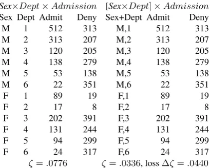
[image:2.595.329.532.375.435.2]

The Berkeley admissions data of Bickel et al. [5] have been intensively studied by many authors, because they show a clear gender bias in the total data; a bias that vanishes when the departments are taken into account. These data may serve as a first demonstration of the use of uncoupling.

Table 1.Berkeley data: Demonstrating Uncoupling of Gender and Depart-ment.

Sex×Dept×Admission [Sex×Dept]×Admission

Sex Dept Admit Deny Sex+Dept Admit Deny

M 1 512 313 M,1 512 313

M 2 313 207 M,2 313 207

M 3 120 205 M,3 120 205

M 4 138 279 M,4 138 279

M 5 53 138 M,5 53 138

M 6 22 351 M,6 22 351

F 1 89 19 F,1 89 19

F 2 17 8 F,2 17 8

F 3 202 391 F,3 202 391

F 4 131 244 F,4 131 244

F 5 94 299 F,5 94 299

F 6 24 317 F,6 24 317

ζ=.0776 ζ=.0336, loss∆ζ=.0440

[image:2.595.75.280.379.543.2]

The two tables in table 1, one the original2×6×2, the other(2×6)×2with gender and department uncoupled, con-tain the same2×6×2 = 24cell frequencies, no variable was summed out or aggregated. This maintenance of the com-plete original data is the salient feature of uncoupling, mak-ing it preferable to aggregation. As uncouplmak-ing only removes the dependence between uncoupled variables and keeps all data intact, this method complies with Fisher’s [6] demand to use all of the data, not aggregated sub-tables: ”In inductive reasoning the whole of the data, or the available axioms, or the available observations, has to be taken into account.” The result of Uncoupling’s analysis in table 2 is very concise:

Table 2.Unraveling the Berkeley Admissions Data.

Zeta for the full table is .0776

∆ζ %Loss Uncoupled variables .0440 57 Dept Gender .0300 39 Dept Admit .0008 1 Gender Admit

We find a strong Department × Gender interaction: women tend to apply to other departments than men. There is

also a strongDepartment×Admissioninteraction: depart-ments differ strongly in their admissions rate. TheGender×

Admissioninteraction is too small to be worth mentioning; the gender bias observed when departments were summed out was due to confounding.

2 Some applications

The following exemplary applications to a number of dif-ferent types of study are intended to indicate the wide range of applicability. They should make the reader familiar with the method and its implications.

2.1 Drug Use of High School Seniors

A study on drug use (A=alcohol, a=no; C=cigarettes, c=no; M=marijuana, m=no) of male and female and white and non-white students (cited from Agresti [7], found the data of table 3. We see a clear preponderance over expec-tation for the complete pattern of abstinence (acm) and the complete pattern of drug use (ACM), the only mixed pattern with an observed count higher than expectation is Acm, the use of alcohol only.

Table 3.Agresti: Drug Use of High School Seniors

White Other Total Total

Female Male Female Male Observed Expected

acm 117 133 12 17 279 ↑ 64.9

acM 1 1 0 0 2 47.3

aCm 17 17 1 8 43 124.2

aCM 1 1 1 0 3 90.6

Acm 218 201 19 18 456 ↑ 386.7

AcM 13 28 2 1 44 282.1

ACm 268 228 23 19 538 740.2

ACM 405 453 23 30 911 ↑ 540

[image:2.595.338.522.532.736.2]

Uncoupling’s analysis of terseness in table 4: for the full table, ζ = .0995. Uncoupling the triple of all three stances accounts for 96% of the terseness, and the three sub-stantial pairwise effectsC×M,A×C, andA×M are all concerned with correlations between substances used.

Table 4.Agresti: Uncoupling triples and pairs of variables.

Terseness of the full tableζ=.0995 ∆ζ %Loss Uncoupled Triples and Pairs

.0952 96 A C M .0474 48 C M Gender .0470 47 C M Race .0193 19 A C Race .0193 19 A C Gender .0105 11 A M Race .0104 11 A M Gender .0026 3 A Race Gender .0023 2 M Race Gender .0019 2 C Race Gender

.0457 46 C M .0178 18 A C

.0085 9 A M

.0014 1 A Race .0013 1 M Gender .0009 1 A Gender .0008 1 C Race .0008 1 C Gender .0007 1 Gender Race .0004 0 M Race

As gender and race do not enter any of the substantial pair-wise effects, one could simply eliminate these two control variables from the final model to obtain a final result of Un-coupling’s analysis: C×M, A×C, A×M.

[image:2.595.334.526.533.739.2]

(3)

an uncoupled composite variablegender×race= [White-Female, WhiteMale, other[White-Female, otherMale], and cross-tabulated it withusagepattern =[acm,. . . ,ACM]. I judged the resulting separabilityγ=.006for predictingusage pat-tern from gender×race to be small enough to be ignored, althoughχ2still indicated a significant difference from zero. In his log-linear analysis using G2 for model selection, Agresti arrived at a more complex model, as many terms were statistically significant, even when an effect was of negligi-ble importance. His reduced model is A×C, A×M, C×M, A×Gender, A×Race, M×Gender, Race×Gender.

A log-linear analysis with SPSS [8], using their automated model selection procedure, resulted in a different model: A×C×Race×Gender, A×M, C×M×Gender, M×Race.

Both Agresti’s and SPSS’s model selections are perfectly admissible, but produce quite different results. As one is free, e.g., to either eliminate one interaction after the other or to eliminate all third order interactions in one sweep, the result of an investigator’s model selection becomes subject to his personal judgment and less objective.

Uncoupling orders the effects along an unequivocal scale of correlation instead of significance tests and does not need subjective decisions, it only needs a specified minimum of an effect size or a ”smallest meaningful difference” and uses the size of terseness∆ζ in reducing the saturated model to arrive at a meaningful parsimonious set of variables and in-teractions, namely C×M, A×C, and M×A.

One may ask why the concept of the smallest meaningful effect is hardly ever used in testing hypotheses or in parsing the saturated model in log-linear analysis, although we all are familiar with it in the context of power calculations.

Uncoupling’s subsequent post factum significance testing has no consequence for model building, it merely makes us aware that an apparently strong effect may not be strong enough with a feeble sample size, or, as in the case of these data, a feeble effect is exaggerated by a large sample.

The choice is:

- with Uncoupling, just a few lines of unequivocal program output

- or lengthy operations with traditional methods, filling many pages of output in sequential simplifications of the sat-urated model, where another researcher may reach different conclusions without committing any error.

2.2 A Problem too Hard for Logistic

Regres-sion

In a flyer advertising Cytel’s LogXact [9] program for ex-act solutions of logistic regression the following problem is presented:

”Diaphragm Use and Urinary Tract Infection. 130 college women with urinary tract infections were compared to 109 matched, uninfected controls. How is urinary tract infection related to age and contraceptive use?”

Woman’s age<24 Y Y Y Y Y Y Y Y Y Y Y Y Y Y N N N N N N N N N N

Used oral contraceptive N N N N N N Y Y Y Y Y Y Y Y N N N N N N Y Y Y Y

Used condom N Y Y Y Y Y N N N Y Y Y Y Y Y Y Y Y Y Y N N Y Y

Used lubricated condom N N N Y Y Y N N N N N N Y Y N N N Y Y Y N N N Y

Used spermicide Y N Y N Y Y N N Y N N Y N Y N Y Y N Y Y N Y N Y

Used diaphragm N N N N N Y N Y N N Y N N N N N Y N N Y N N N N

Infected 1 14 3 10 12 1 44 3 0 15 1 2 7 3 2 1 1 1 0 1 5 0 3 0

Total 2 16 4 18 30 1 86 3 1 16 1 2 12 9 2 1 1 3 4 1 19 1 4 2

How to read this table: The first column on the left tells us that there were 2 women total (1 infected) with these characteris-tics: Age<24, did not use oral contraceptive, did not use condom, did not use lubricated condom, did use spermicide, and did not use diaphragm.

”Challenge: Try fitting a logistic regression model to these data with all six covariates included. Conventional asymp-totic logistic regression cannot meaningfully fit this model when the variable for diaphragm use is included. Only the exact methods in LogXact 4 can pin down the effect of this potentially important variable”..

Clearly, this data set poses difficulties, as the frequency table is rather sparse, only 44 of the possible 27_{=128 cell}

frequencies are greater than zero. More difficulty stems from the perfect discrimination ofdiaphragmandinfection.

Where a standard logistic regression found no solution for the variablediaphragmand LogXact was able to arrive at a solution identifyingdiaphragm as a significant predictor of urinary tract infection, Uncoupling had no problem whatso-ever finding a solution when I took the challenge; just like LogXact it identified diaphragm as an important predictor. Uncoupling’s simple and robust computation ofζ does not contain any iterative algorithm that may converge slowly or not at all.

2.3 Radelet’s Death Penalty Data

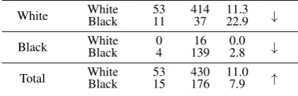
[image:3.595.310.521.414.482.2]

A well-known problem is Radelet’s study (cited from Agresti [7]) on Florida death penalties influenced by the defendant’s race when controlling for the victim’s race as shown in table 5.

Table 5.Radelet: Frequency of Death Penalty in Florida.

Race of ... Y=Penalty

X1=VictimX2=Defendant Death No death Percent Death

White White_Black 53₁₁ 414₃₇ 11.3_22.9 ↓

Black White_Black 0₄ ₁₃₉16 0.0_2.8 ↓

Total White_Black 53₁₅ 430₁₇₆ 11.0_7.9 ↑

If the victim was white, black defendants received a death penalty more often than white defendants, and this was also the case when the victim was black. Yet, when collapsing the table by ignoring the victim’s race (summing out the victim’s race), in the total white defendants received the death penalty more often (cf. the arrows in table 5).

The primary question was: “How strongly does the color of the defendant determine the penalty?”, and we get two conflicting answers when we compare the total result with the result within victims’ race. The puzzling reversal of trend in the collapsed table is known as Simpson’s paradox, a phe-nomenon that cannot occur in designed experiments where all variables are orthogonal to each other.

In this low-dimensional example Simpson’s paradox was recognizable by visual inspection of the cross-tabulation. In the analysis with Uncoupling the non-orthogonality is more quickly detected by studying the∆ζin table 6 :

Table 6.Radelet: Terseness when uncoupling pairs of Variables.

Terseness of full tableζ=.2577 ∆ζ %Loss Pairs of uncoupled Variables .2436 95 Defendant Victim

.0131 5 Victim Penalty .0034 1 Defendant Penalty

Whereas the terseness of the complete table was ζ = .2577, uncouplingX1=defendant andX2=victim reduces the

(4)

Black defendants tend to have killed black victims and white defendants tend to have killed white victims, and this non-orthogonality produces the baffling paradox.

This annoying interdependence of X1 and X2 is

elimi-nated by uncoupling, combining the values ofX1 (race of

defendant) andX2(race of victim) into a composite variable victim/defendant= [W/W,W/B,B/W,B/B] to remove any de-pendence.

Terseness is reduced to justζ=.0141for the2×[2×2] table in whichX1andX2are uncoupled. We should revise

our original question and ask: “How is the sentence deter-mined by the composite of victim’s and defendant’s race?”. The separabilityγsentenceof predicting the death sentence

us-ing the composite variable isγ=.0505, and this answers the revised question. We might go on to look at white and black defendants only and find thatγsentenceis a rather small .0113

for white defendants versus a strong .1612 for black defen-dants. The black defendant’s sentence is strongly influenced by the race of his victim. This finding is rarely mentioned in published analyses.

It is our conviction that the summing out of the con-trol variableX2=victim, in an effort to produce a summary,

amounts to an illegal act that produces Simpson’s paradox (cf. Fisher’s demand above [6]). In this extreme case, where summing out produced the paradox, you will probably agree, but I would like to propose a general rule banning the sum-ming out of control variables when they are involved in a sizeable∆ζ effect. The error involved in collapsing tables when an effect is insignificant, routinely done in parsing log-linear models, is only gradually less severe than when a very largeXi–Xj–relationship produces Simpson’s paradox.

2.4 Byssinosis, an epidemiological example

[image:4.595.83.272.526.670.2]

Let us now turn to a complex data set with six variables by Higgins and Koch [10] as shown in table 7.

Table 7.Byssinosis by Employment, Smoking, Gender,Race and Dustiness.

Dustiness of Workplace most medium least Employ Smoke Sex Race No Yes p No Yes p No Yes p

<10

Yes M

white 37 3 .08 74 0 .00 258 2 .01 other 139 25 .15 88 0 .00 242 3 .01 F white_other ₂₂5 0₂ .00_.08 ₁₄₅93 1₂ .01_.01 ₂₆₀180 ₃3 .02_.01

No M

white 16 0 .00 35 0 .00 134 0 .00 other 75 6 .07 47 1 .02 122 1 .01 F white_other ₂₄4 0₁ .00_.04 ₁₄₂54 1₃ .03_.02 ₃₀₁169 ₄2 .01_.01

10-20

Yes M

white 21 8 .28 50 1 .02 187 1 .01 other 30 8 .21 5 0 .00 33 0 .00 F white_other 0₀ 0₀ ??_?? 33₄ ₀1 .03_.00 94₃ ₀2 .02_.00

No M

white 8 2 .20 16 1 .06 58 0 .00 other 9 1 .10 0 0 ?? 7 0 .00 F white_other 0₀ 0₀ ??_?? 30₄ ₀0 .00_.00 90₄ ₀1 .01_.00

≥20

Yes M

white 77 31 .29 141 1 .01 495 12 .02 other 31 10 .24 1 0 .00 45 0 .00 F white_other 1₁ 0₀ .00_.00 91₀ ₀3 .03_?? 176₂ ₀3 .02_.00

No M

white 47 5 .10 39 0 .00 182 3 .02 other 15 3 .17 1 0 .00 23 0 .00 F white_other 2₀ 0₀ .00_?? 187₂ ₀3 .02_.00 340₃ ₀2 .01_.00

The complete3×3×2×2×2×2table is difficult to assess. When one tries to find the main factors leading to byssinosis, a lung disease caused by exposure to cotton dust, one has to take into account many interrelations between the possibly illness-inducing variables. Higgins and Koch de-vised a laboriousχ2-based set of rules designed to find the important factors; they concluded that dustiness of the work-place is the most important determinant of illness, gender of employee is 2nd, and smoking is in 3rdplace. From the con-tent of the study, it seems curious that the length of employ-ment and therefore the length of exposure to dust came in 4th_{place only. Could it be that some confounding relation}

has suppressed the relation between length of exposition and byssinosis? The∆ζ in table 8 should provide an answer to this question.

Table 8.Byssinosis: Terseness when uncoupling pairs of Variables.

Terseness of the full tableζ=.0984 ∆ζ %Loss Pairs of uncoupled Variables .0486 49 Race, Employment length .0137 14 Gender, Dust

.0102 10 Gender, Smoker .0066 7 Race, Dust

.0060 6 Gender, Employment length .0057 6 Byssinosis, Dust

.0027 3 Smoking, Employment length .0027 3 Dust, Employment length .0026 3 Race, Gender

.0009 1 Byssinosis, Employment length .0008 1 Smoker, Dust

.0006 1 Byssinosis, Smoker .0006 1 Race, Smoker .0005 1 Byssinosis, Gender .0003 0 Byssinosis, Race

Reassuringly, the order of pairs that includebyssinosisis 1stdust, 2ndlength of employment, and 3rdsmoking. This appears more plausible for a lung disease.

But the largest∆ζ occurs for the uncoupling of race and length of employment, which is responsible for almost half of the tersenessζ=.0984 of the whole table, non-whites have a much higher turnover.

This non-orthogonality has the effect that the clear increase of byssinosis with length of employment (and therefore ex-posure) seen within race is reduced when race is summed out (table 9).

Table 9.% of Byssinosis within race vs Total.

Employment White Other Total

<10 1.12 3.08 2.31 10 to 19 2.81 8.33 3.65

≥20 3.42 9.49 3.84

Here, the collapsing of the table by summing out race was not yet an error producing a reversal of trend as in Simpson’s paradox, but it is an error that led Higgins and Koch to un-derestimate the effect of length of exposure on developing a byssinosis, producing an ”attenuated Simpson”.

The error of summing out will affect any of the statistical models usually applied in the analysis of data, as in the last resort they all use summaries of partially collapsed tables to arrive at their estimates of main effects. Fortunately, collaps-ing of tables by summcollaps-ing out variables is not needed; un-coupling can successfully replace it without producing con-founding results, as it does not discard data but merely rear-ranges them.

3 A program for the analysis

A program Uncoupling(Windows) is available from the author that starts by computing the separabilitiesγwith each variable in turn regarded as the dependant variable.

In the main part, tersenessζis computed with all pairs and higher tuples of variables uncoupled. All combinations of variables are analyzed.

(5)

Optionally, one can request bootstrapped error estimates.

Acknowledgements

This paper and the program could never have been written without the seminal work that Lucien Preuss has compiled over the years, letting me participate. I must take full respon-sibility for the presentation, however.

Thanks is also due to Christoph E. Minder who carefully read an earlier manuscript and made me aware of several in-consistencies.

REFERENCES

[1] Preuss, Lucien and Vorkauf, Helmut:The Knowledge Content of Statistical Data.Psychometrika, 1997,Vol 62, No 1, 133-161

[2] Preuss, Lucien:A class of statistics based on the information concept.Communications in Statistics - Theory and Methods, 1980,Volume 9, Issue 15

[3] Kruskal, William and Majors, Ruth:Concepts of relative Im-portance in Recent Scientific Literature.The American Statis-tician, February 1989, Vol. 43, No. 1

[4] Press, William H., Flannery, Brian P., Teukolsky, Saul A., Vet-terling, William T.: Numerical Recipes: the Art of Scientific Computing3rd ed., Cambridge University Press, 1992,p. 761.

[5] Bickel PJ, Hammel EA, O’Connell JW:Sex Bias in Graduate Admissins: Data from Berkeley.Science, 1975, Vol 187, 398-404.

[6] Fisher, R. A.:The Nature of Probability. Centennial Review, 1958, v. 2, 261-274

[7] Agresti, Alan: Categorical Data Analysis. Wiley, 2002 a)

Drug Use, pp 322-326, 361-363, 367, 482-483, 528 b)Death Penalty, pp 48-52, 63, 65, 201

[8] SPSS Inc: SPSS Statistics for Windows, Version 17.0. Chicago: SPSS Inc.

[9] Cytel Inc: LogXact 8.675 Massachusetts Ave., Cambridge, MA 02139-3309