Incompressible fluid flow and energy equations simulation on distributed parallel computer system

INCOMPRESSIBLE FLUID FLOW AND ENERGY EQUATIONS SIMULATION ON DISTRIBUTED PARALLEL COMPUTER SYSTEM

Manshoor. B1, Wan Hassan, M.N2, Alias. N3

1

Faculty of Mechanical & Manufacturing Engineering Universiti Tun Hussein Onn Malaysia, Batu Pahat, Johor

2

Faculty of Mechanical Engineering Universiti Technologi Malaysia, Skudai, Johor

3

Faculty Science

Universiti Technologi Malaysia, Skudai, Johor

ABSTRACT

This paper is concerned with the development of an efficient scheme for solving the finite difference Navier-Stokes and energy equations using distributed parallel computer system. The numerical procedure is based on SIMPLE (Semi Implicit Method for Pressure Link Equations) developed by Spalding. The hybrid scheme which is combination of the central difference and up wind scheme is used in obtaining a profile assumption for parameter variations between the grids points. Parallelization method used on this distributed parallel computer system is Domain Decomposition Method (DDM). The accuracy of the parallelization method is done by comparing with a benchmark solution of a standardized problem related to the two dimensional buoyancy flow in a square enclosure.

Keywords: simple algorithm; parallel algorithm; domain decomposition method; navier-stokes equations

INTRODUCTION

Parallel computing or also known as parallel processing refers to the concept of speeding up the excitation of a program using multiple processors by dividing the program into multiple fragments that can execute simultaneously, each on its own processor. A program being executed across n processors might execute n times faster than it would use a single processor. Here we can say that the parallel processing is differs from multitasking in which a single processor execute several programs at once.

incompressible flow become more complicated and need a high performance computer to solve the problem.

To overcome this problem, parallel computer was used and to determine the performance of this parallel computations, the corresponding parallel algorithms was developed and it based on method of parallelization known as Domain Decompositions Method. Control volume approach is selected and the matrix formed will solved using matrix tri-diagonal solver.

GOVERNING EQUATIONS

Two-dimensional incompressible laminar constant-density flow and energy equation is governed by set of partial differential equations (M.C.Melaaen, 1993). The continuity, momentum and energy equations in their primitive form are shown in equations (1-4) where the equation for conservation of mass is given by:

=

0

∂

∂

+

∂

∂

y

v

x

u

The conservation of momentum in x and y directions are governed by the u -momentum equation expressed as:

S_u y u x u x P y u v x u

u _⎟⎟+

⎠ ⎞ ⎜⎜ ⎝ ⎛ ∂ ∂ + ∂ ∂ + ∂ ∂ − = ∂ ∂ + ∂ ∂ 2 2 2 2 1

ρ

µ

ρ

as well as the v-momentum equation:

S_v y v x v y P y v v x v

u _⎟⎟+

⎠ ⎞ ⎜⎜ ⎝ ⎛ ∂ ∂ + ∂ ∂ + ∂ ∂ − = ∂ ∂ + ∂ ∂ 2 2 2 2 1

_ν

ρ

The conservation of energy express as:

_⎟⎟ ⎠ ⎞ ⎜⎜ ⎝ ⎛ ∂ ∂ + ∂ ∂ = ∂ ∂ + ∂ ∂ 2 2 2 2 y T x T c k y T v x T u P

ρ

DISCRETISATION

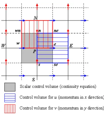
In order to numerically solve the velocity and pressure fields that obey the discretized momentum and continuity equations, the finite difference method was applied. This method involves integrating the continuity and momentum equations over a two-dimensional control volume on a staggered differential grid shown in Figure 1 (S.V.Patankar and D.B.Spalding, 1972).

This yields the governing equations in their discretized form as shown in equations (5-6). The staggered grid evaluates the scalar variables, in this case only the pressure, which are stored at the scalar nodes and located at the intersection of two unbroken grid lines. The u-velocity components are stored at the east and west cell faces of the scalar control volume and are indicated by the lower case letters e and w. The v-velocity components are stored at the north and south cell faces of the scalar control volume which are indicated by the lower case letters n and s. These velocity components are located at the intersection of a dashed and unbroken line that construct the scalar cell faces and are indicated by arrows.

FIGURE 1 Staggered Grid showing locations of flow variables

The horizontal arrows shown indicate the locations of the ue and uw velocity components and the vertical arrows indicate the locations of the vn and vs velocity components. After the process of discretization, the discretized of u-momentum equation becomes:

a_i,_Ju*_i,_J =

∑

(

)

and discretized of v-momentum equation becomes:

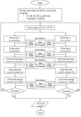
SOLUTION PROCEDURE OF THE SIMPLE ALGORITHM

The SIMPLE method proceeds by a cyclic series of guess and correct operations. The flow chart of the algorithm showed in Figure 2. Treat the corrected pressure p

as new guessed p*, return to step 2 and repeat the whole procedure until a

converged solution is obtained.

PARALLEL IMPLEMENTATION

A parallel implementation can provide a further reduction in computing time. Parallel implementation also makes solution possible to problems that would require too much memory to solve on a single processor. During to solve this problem, the parallel implementation is based on message passing (distributed memory systems) using the Parallel Virtual Machine (PVM) software. Portability is ensured because PVM is available on many types of parallel computers.

The implementation uses a layer of subroutines on top of PVM, symbolically denoted by start: start entire parallel application, stop: stop parallel application,

send: send a message and receive: receive a message.

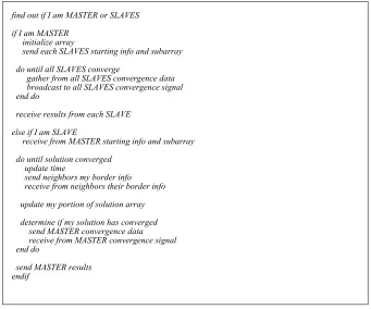
Communication process is the most important process in parallel implementation. For the send and receive subroutines, it consists of communication process between a data or function that will be send or receive. According to the pseudo code solution in Figure 3, the communication process occurs between the master and slave during to their sending and receiving the data or function.

find out if I am MASTER or SLAVES

if I am MASTER initialize array

send each SLAVES starting info and subarray

do until all SLAVES converge

gather from all SLAVES convergence data broadcast to all SLAVES convergence signal end do

receive results from each SLAVE

else if I am SLAVE

receive from MASTER starting info and subarray

do until solution converged update time

send neighbors my border info receive from neighbors their border info

update my portion of solution array

determine if my solution has converged send MASTER convergence data receive from MASTER convergence signal end do

send MASTER results endif

COMMUNICATION

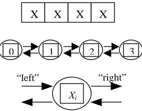
Basically this finite difference problem is same with the solution of the problem in this project. From top to bottom of the Figure 4; the one-dimensional vector X, where N=4; the task structure, showing the 4 tasks, each encapsulating a single data value and connected to left and right neighbors via channels; and the structure of a single task, showing its two inports and outports.

FIGURE 4 A parallel algorithms for the finite difference problem

We first consider a one-dimensional finite difference problem, in which

we have a vector

X

X

( ) ( ) ( ) ( )

4 2 :

0 , 1

0 1 1

t i t i t i t i

X X X

X T t N

i_{< − ≤ <} + ₌ + + + <

That is, we must repeatedly update each element of X, with no element being updated in step t+1 until its neighbors have been updated in step t. A parallel algorithm for this problem creates N tasks, one for each point in X. The ith task is

given the value

X

valuesX_i( )1, X_i( )2 ,..., X_i( )T .

Hence, at step t, it must obtain the values X_i−1( )t and

( )t i

X +1 from tasks i-1

and i+1. We specify this data transfer by defining channels that link each task with “left” and “right” neighbors, as shown in Figure 4, and requiring that at step

t, each task i other than task 0 and task N-1.

i. sends its data X_i( )T on its left and right outports, ii. receives X_i−1( )t and

( )t i

X +1 from its left and right inports, and

iii. use these values to compute X_i( )t+1 .

Notice that the N tasks can execute independently, with the only constraint on execution order being the synchronization enforced by the receive operations. This synchronization ensures that no data value is updated at step t+1 until the

X X X X

0 1 2 3

Xi

data values in neighboring tasks have been updated at step t. Hence, execution is deterministic.

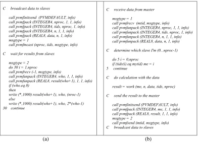
Figure 5(a) and 5(b) below showed the algorithms for the sending and receiving data from master and slaves.

C broadcast data to slaves

call pvmfinitsend (PVMDEFAULT, info) call pvmfpack (INTEGER4, nproc, 1, 1, info) call pvmfpack (INTEGER4, tids, nproc, 1, info) call pvmfpack (INTEGER4, n, 1, 1, info) call pvmfpack (REAL8, data, n, 1, info) msgtype = 1

call pvmfmcast (nproc, tids, msgtype, info)

C wait for results from slaves

msgtype = 2 do 30 i = 1,nproc

call pvmfrecv (-1, msgtype, info)

call pvmfunpack (INTEGER4, who, 1, 1, info) call pvmfunpack (REAL8, result(who+1), 1, 1, info) if (who.eq.0)

then

write (*,1000) result(who+1), who, (nroc-1) else

write (*,1000) result(who+1), who, 2*(who-1) 30 continue

C receive data from master

msgtype = 1

call pvmfrecv (mtid, msgtype, info)

call pvmfunpack (INTEGER4, nproc, 1, 1, info) call pvmfunpack (INTEGER4, tids, nproc, 1, info) call pvmfunpack (INTEGER4, n, 1, 1, info) call pvmfunpack (REAL8, data, n, 1, info)

C determine which slave I'm (0...nproc-1)

do 5 i = 0,nproc if (tids(i).eq.mytid) me = i 5 continue

C do calculation with the data

result = work (me, n, data, tids, nproc)

C send the result to the master

call pvmfinitsend (PVMDEFAULT, info) call pvmfpack (INTEGER4, me, 1, 1, info) call pvmfpack (REAL8, result, 1, 1, info) msgtype = 2

call pvmfsend (mtid, msgtype, info) C broadcast data to slaves

(a) (b)

FIGURE 5 Algorithm master to send and receive data to and from slaves and algorithm slaves to receive and send data from and to master

VALIDATION OF THE RESULTS

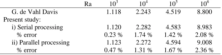
Tables 1 to 3 show the comparison between the results from the present simulation and the literature results obtained by de Vahl Davis. The results of de Vahl Davis are the standards against which all other codes are evaluated. Maximum horizontal velocity on the vertical midplane of the cavity, Umax, maximum vertical velocity on the horizontal midplane of the cavity, Vmax, and an average of Nusselt number were compared at Rayleigh numbers of 103, 104, 105 and 106. The comparison had been done between the benchmarking results obtained by de Vahl Davis which in serial processor and the present study that are simulation using serial processor and parallel processor or parallel computer.

methods of solution was below than 3% compare with benchmark result. Besides that, the result that was showed in the forms of contour maps of non-dimensional temperature and velocities was also compared with the results that obtained by de Vahl Davis.

TABLE 1 Comparison of the numerical result of present study for Umax

Ra 103 104 105 106

G. de Vahl Davis 3.649 16.193 34.620 64.593

Present study:

i) Serial processor 3.652 16.163 34.871 65.812

% error 0.082 % 0.185 % 0.725 % 1.880 %

ii) Parallel processor 3.592 16.376 34.852 65.847

% error 1.560 % 1.131 % 0.670 % 1.941 %

TABLE 2 Comparison of the numerical result of present study for Vmax

Ra 103 104 105 106

G. de Vahl Davis 3.697 19.167 68.590 216.360

Present study:

i) Serial processing 3.704 19.675 69.482 220.641

% error 0.189 % 2.650 % 1.300 % 1.978 %

ii) Parallel processing 3.715 19.642 69.680 221.282

% error 0.487 % 2.478 % 1.589 % 2.275 %

TABLE 3 Comparison of the numerical result of present study for

____

Nu

Ra 103 104 105 106

G. de Vahl Davis 1.118 2.243 4.519 8.800

Present study:

i) Serial processing 1.120 2.282 4.583 8.983

% error 0.23 % 1.74 % 1.42 % 2.08 %

ii) Parallel processing 1.123 2.272 4.594 9.008

% error 0.47 % 1.31 % 1.67 % 2.36 %

PARALLEL COMPUTING RESULTS

communication time. Table 4 showed the result of execution time between sequential and parallel solution and the tabulated results of computational time and communication time.

TABLE 4 Execution time for computational solutions

Sequential time Parallel time tcomp tcomm tp

Ra.

no

103 32.8 s 9.43 s 8.41 s 1.02 s 9.43 s

104 135.75 s 41.39 s 34.62 s 6.78 s 41.39 s

105 2040.26 s 612.06 s 522.82 s 89.24 s 612.06 s

106 163602.04 s 49080.61 s 41923.02 s 7157.60 s 49080.61 s

Execution time is not always the most convenient metric by which to evaluate parallel algorithm performance. As execution time tends to vary with problem size, execution times must be normalized when comparing algorithm performance at different problem sizes.

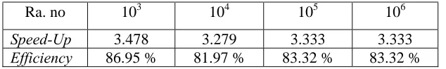
Other parameter that was used to measure a performance of parallel computations is speed-up and efficiency. From the speed-up, we know that how fast the parallel computer solves the problem under consideration. It is sometimes useful to know how long processors are being used on the computation, which can be found from the efficiency.

TABLE 6Results for speed-up and efficiency

Ra. no 103 104 105 106

Speed-Up 3.478 3.279 3.333 3.333

Efficiency 86.95 % 81.97 % 83.32 % 83.32 %

DISCUSSION AND CONCLUSION

From the results that were obtained, we can see that execution time for parallel computation was decrease compare with sequential computation. By using sequential computation, total execution time that we need to complete our

simulation at Rayleigh number 106 is 163602.04 seconds or 2726.7 minutes or

45.45 hours. For parallel computation, we were reduced an execution time for the

simulation at Rayleigh number 106 to 49080.61 seconds or 818.01 minutes or

13.63 hours. In theory, by using 4 processors to solve this problem, we can reduce an execution time until 75%. However, it cannot be achieved since the communication process was occurring.

with the benchmark result. Thus, the simulation is successful. Percentage errors for the computational solution which are simulation by serial and parallel computer are below than 3% compare with benchmark result by de Vahl Davis. Therefore it has proved that clustering personal computers together can provide adequate computing power for large engineering problems.

REFERENCES

Date A. W (1985). “Numerical Prediction of Natural Convection Heat Transfer in Horizontal Annulus.” Int. J. Heat Mass Trasfer.

Davis G. de Vahl (1983). “Natural convection of air in a square cavity: a

benchmark numerical solution”. Int. Journal Numerical Mech. Fluid 3:

249-264.

Dongarra, J. & Eijkhout, U. (2000). “Numerical linear algebra algorithms and

software.” Journal of Computational and Applied mathematics. 123(2):

489-514.

Geist, A. et al. (1994). “PVM: Parallel Virtual Machine. A Users’ Guide and Tutorial for Networked Parallel Computing”. Massachusetts: The MIT Press.

Patankar S. V (1980). “Numerical Heat Transfer and Fluid Flow.” McGraw-Hill Inc, New York.

Patankar S.V and Spalding D. B (1972). “A Calculation Procedure for Heat, Mass

and Momentum Transfer in 3-Dimensional Parabolic Flows.” Int. J. Heat

Mass Trasfer.

Spalding D. B (1972). “A Novel Finite Difference Formulation for Differential

Expressions Involving Both First and Second Derivatives.” Int. J. Num.

Methods Eng. 3: 551-559.