Fast Laser Spectroscopy: Dynamical Absorption Line
Igor Peshko
Department of Physics and Computer Science, Wilfrid Laurier University, 75 University Ave West, Waterloo, Ontario, N2L 3C5, Canada *Corresponding Author: [email protected]
Copyright © 2014 Horizon Research Publishing All rights reserved.
Abstract
This paper presents analysis of the problems and principles of design of the remote, fast, and precise spectroscopic sensor, operating from the robotic platform. The typical errors of gas concentration measurement have been analyzed. It has been shown that in case of fast tunable laser spectroscopy (a sample registration time – 100ns or less) the line shape is, in principle, unrepeatable, asymmetric, and chaotically modulated at each new scan. The final composite line profile is sharper at the top as compared with a Lorentzian one and wider near the bottom. Three reasons for such specific line shape formation were considered: 1) The gas absorption line shape has been simulated by the summation of Lorentzian lines of different linewidth. The Maxwellian distribution of the molecular speeds has been used to find the molecular collisional energy distribution and related linewidths with taking into account probable number of molecules with specific impact energy; 2) Appearance of the spectral satellites when the absorption process is suddenly interrupted; 3) Spectral presentation of the collision correlation function that is modulated by massive collisions at free-flight termination. To calculate the gas concentration properly the data received from the independent sensors of pressure, temperature and humidity have been used.Keywords
Laser Spectroscopy, Absorption Line Shape, Model of Absorption Line Formation, Spectroscopic Sensor, Gas Concentration Measurement1. Introduction
1.1. General Background
The strategic task of modern gas sensory technology is the design of accurate remote sensor, capable of evaluating several gases during a few seconds in changeable and uncontrollable conditions, without calibration, and operating from the robot. This paper is the third chapter in the “Smart Sensory Spectroscopy” series. In the first paper [1], basic principles of design and operation of a multifunctional scientific instrument, based mainly on the spectroscopic principles, have been considered. Single-frequency, tunable diode lasers have been used to operate a multifunctional
device that combined the functionalities of a spectrometer, rangefinder, gas sensor, sensor calibrator, and spectroscopic isotope identifier. In second paper [2] the oxygen remote sensor has been described. It has demonstrated unprecedented accuracy (error less than 1%) in combination with immediate response.
In this paper the reasons of measurement errors that can be generated in process of gas concentration evaluation are analyzed. The spectral line strength and linewidth are typically used to estimate the gas concentration. However, just these two parameters are not sufficient for precise measurements, especially if data acquisition time is just nanoseconds. The knowledge of true line shape and dynamical variations of this shape contains crucial information for correct gas concentration estimation.
To perform the gas concentration measurement fast and remotely the only one possibility is to use photonic technology. Spectroscopy is successfully applied in analysis of content of faraway located objects, like stars or nebulas. However, providing a fast and precise quantitative measurement is not a simple task. The commercially available portable spectrometers are typically failed in case of simultaneous action of several chemical agents: the fast recognition of dangerous gases in presence of even non-toxic background gases that somehow deform the spectrum view of specific substance is a big problem.
All theoretical profiles are typically analyzed and compared with experimentally observed lines, achieved in slowly operating high-resolution spectrometers. These instruments provide averaging of the signals during tens of minutes. However, the chemical identifier must react in fractions of a second. The question is what will happen if the registration time is nanoseconds, the laser beam path length is just centimeters, the laser beam cross-section diameter is a few hundred microns, and the spectral width of the laser radiation line is much narrower than the absorption line width? The attempts to answer these questions are presented in this paper.
1.2. Spectroscopic Sensory Techniques
radiation); b) Chemical Agents (CA); c) Toxic Industrial Chemicals (TIC/ or TIM – Toxic Industrial Materials); d) Volatile Organic Compounds (VOC), e) Radiological Hazards Detection: α-, β-, and γ-radiation, X-ray, and neutron fluxes (RH); f) Explosive Materials (EM); and g) Biological Hazards (BH).
The absorption spectroscopy remote gas sensor discussed in this paper is aimed to recognize the gases or vapors and to estimate concentration of any substances that have absorption bands in visible and IR ranges where appropriate lasers are available. The oxygen near-IR absorption bands were used as a model structure to investigate the peculiarities of the dynamical line shape at ultra-fast data acquisition.
The successfully operating reconnaissance robot cannot be designed as a simple mechanical combination even of well working commercial devices because of weight, size, and power consumption limitations. Moreover, currently available sensory technologies sometimes cannot operate properly when closely located or affected by specific conditions. For example, the ionizing radiation detector (such as 1703GNB or G20-ER10) can “feel” the radioactive source located in the ion mobility spectrometer (such as SABRE 5000) and could be “blind” detecting low levels of external radiation. Inversely, in the presence of external radiation the ion mobility spectrometer loses the accuracy because of additional external ionization factors. Some chemical agents, e.g. Soman (C7H16FO2P) and Cyclosarin (C7H14FO2P), characterized with very similar chemical formulas, can be identified with errors when detected with standard commercial sensors. The portable spectral sensors typically have a relatively low resolution and can generate error when several chemical agents or compounds with overlapped spectra should be detected.
One way to solve the efficiency and weight/size problem is multi-functionality of the devices: 1) “All-in-one” principle – the same hardware (lasers, sensors, detectors, power supplies, etc.) is used in different devices; 2) “One-for-all” principle – the information acquired from some sensor is cross used by other sensors to improve the accuracy of measurements; different physical processes are used for estimation of specific agent or parameter; 3) “The same band” principle – specification of the spectral band where several substances can be detected by the same sensor. An example of such device is the gas sensor described in [1]. The instrument consists of a multi-functional miniature spectrometer, a multi-gas photonic sensor, rangefinders, isotope identifiers, and sensors of temperature, pressure, humidity, and background radiation. This device is capable to detect CO, CO2, CH4, O2, and H2O vapors, to monitor atmospheric conditions and to scan the environment with laser rangefinders that simultaneously serve the spectral sensor. The bench-top prototype, operated by a Sacher Lasertechnik diode laser, tunable in the range of roughly 1570–1670 nm [3] can additionally detect N2O, HI, OH radicals, and C2H2.
Potentially, several spectroscopic techniques can be used
from a robotic platform: 1) cavity ring-down spectroscopy (CRD), 2) frequency modulation spectroscopy (FMS), 3) laser induced breakdown spectroscopy (LIBS), 4) Raman spectroscopy of different types (RS), 5) super-continuum spectroscopy (SCS), and 6) tunable laser spectroscopy (TLS).
1) CRD spectroscopy is a sensitive absorption technique in which the rate of light pulse absorption is measured. The sample is placed inside a high-finesse optical cavity consisting of two highly reflective mirrors. In this way the rate of absorption can be obtained; the more the sample absorbs, the shorter is the decay time [4-6]. Unfortunately, in the presence of mechanical vibrations and variations in atmospheric conditions, the system cannot operate properly.
2) A variety of FMS methods for high-sensitivity absorption detection of gas-phase species has evolved in recent years. The mathematical derivations of the signals in wavelength-modulation spectroscopy and one- and two-tone frequency-modulation spectroscopy are used for increase of the signal rate and amplitude [7]. Wavelength modulation, traditionally performed at kilohertz frequencies, usually achieves sensitivities of 10−4 – 10−5 [8]. The FM techniques at megahertz frequencies have been used to overcome low-frequency laser noise so that detector-limited sensitivities of the order of 10−7 – 10−8 are possible [9,10]. Unfortunately, the highly sensitive techniques emphasize optical and electrical noise and occasional spikes. The scanning in relatively wide spectral range results in hardly recognizable spectral image.
3) The LIBS is a powerful tool for remote substance identification [11]. However, in our case the robotic platform had very strict weight/size/power consumption limitations and existing models of LIBS device cannot be used in our conditions. Moreover, the laser plasma plume can contain the same ions initially belonged to different molecules and different aggregate states of a substance. Hence, the relative concentration of different agents could be found very approximately.
4) There is a wide variety of RS techniques potentially applicable for Homeland security, civil and medical applications (see a review in [12]). A general problem of these techniques is a weak signal that typically failed at few meters distance or in the presence of some background radiation.
5) SCS [13] typically covers tremendous spectral range in just a single ultra-short laser pulse. However, it requires a wide-band, low-resolution spectrometer to overview the available spectral band. In this case the real area under the absorption line and line width are unknown and the monitored substance concentration cannot be estimated enough precisely.
spectral line shape, width, and line maximum position [14-17]. The systems for gas detection in the middle-infrared range were demonstrated in [18-20]. These publications were focused mainly on the new diode laser development and have not discussed the field sensor problems.
The well-developed sensors are industrial ones that operate in known ranges of repeatable conditions with some specific substances and possibility of periodical calibration. Most of the oxygen sensors used for industrial and environmental applications exploits different types of interactions between oxygen and testing material of the sensor [21]. Hence, all of them are the local measurement technologies. For the remote oxygen sensor different types of tunable diode lasers have been proposed and tested to measure the gas concentration [22].
1.3. Experimental Set-up
The detailed description of the experimental set-up can be found in [1,2]. Here we repeat briefly the list of equipment and the main parameters. The sensor consists of the diode laser with a collimator, a reference detector with a filter and beam splitter, sensors of ambient parameters, a wanted signal detector, an analog signal digitizer, a sensor controller, and batteries. The FDS100 photodiodes have been used as detectors (10-ns rise-time). The signals from different sensors were digitized with a NIUSB-600B (8 inputs, 12-bit, 10kS/s) DAQ. Within the range of approximately 13135 – 13150 cm-1 (760 – 761.3nm), up to nine oxygen sharp lines have been detected. The responsivity of the detector changes at approximately 1.5% along the laser tuning rate around a 761-nm optical wavelength. In our experiments, we used diode laser with a 30 MHz laser linewidths [23]. The absorption spectral linewidth in MHz units is approximately 1500 MHz. Hence, the total line can be represented by scanning through 50–60 points. In other words, 64 time points along the absorption line can realize maximal physical spectral resolution achievable with this type of laser. In our project the total data acquisition time was specified as 1 sec. The total scanned range was 15 cm-1 and a linewidth value was approximately 0.05 cm-1. In case of low signal/noise ratio, the minimal number of scans was 500 [1], the time of single scan was 2 ms, and time of signal accumulation at single spectral point (sample) was 100 ns at 10 Hz laser modulation rate.
1.4. The Line Shape Approximations
The classical spectroscopy typically considers two main types of the absorption line broadening: Gaussian (low gas pressure < 1kPa, high temperature) and Lorentzian (high gas pressure > 100kPa), or their convolution – Voigt (pressure between high/low limits) [24]. Next level models have been developed starting from these basic approximations. The line shape models that include motional Dicke narrowing effects [25], Galatry (soft collision) [26], and Rautian-Sobel’man
(hard collision) [27] profiles yield significant improvements in the spectral line shape fits compared with Voigt profile. In work [18] the spectral line intensities and self-broadening parameters have been determined by fitting the measured spectra with Voigt, Galatry, and Rautian line shape models.
Among the early works the fundamental research [28] should be specially mentioned. In this work the Speed Dependent Voigt Profile has been investigated. The Doppler-shifted Lorentzian line profile for the atoms moving with velocity distributed according with the Maxwellian function has been considered. Moreover, the speed dependent broadening and shift parameters have been introduced to precisely describe the final line asymmetry and shape deviation. The relation between the parameters describing Dicke narrowing with the use of the soft- and hard-collision models has been discussed and verified experimentally in [6]. The HF in an Ar line shape below atmospheric pressure has been investigated in [29, 30]. The line shapes exhibit strong collisional narrowing and a slight asymmetry which has been modeled with hard or soft collision profiles modified for partial correlation between velocity- and state-changing collisions.
In real case both speed-dependent effects and Dicke narrowing should be taken into account. Analytical expression for this kind of profiles can be found in [31 – 33]. Namely, in [33] several processes affecting the line shape were summarized. Numerical calculations show that speed-dependent effects can produce the additional line narrowing as well as broadening and also the line asymmetry. A uniform formula describing the shape in the core and near wings of a spectral line has been proposed. The pressure broadening and shift, Doppler broadening, and collision narrowing, which are described using soft and hard collision models, correlation between pressure and Doppler broadening, and dispersion asymmetry of the line have been taken into account. At last, the density, the mass of the perturber, and the ratio of the optical to kinetic cross section all play a role in revealing or concealing (in the profile) the effects of broadening, which depend upon the speed of the active molecule [34].
spectral lines, which demonstrate maximal shift/narrowing effect were chosen within a total absorption rotational-vibration bands. However, very often even closely located spectral lines demonstrate dramatically different experimental behavior [40]. This is a serious obstacle in the way of creation of the “universal” spectroscopic sensor based on any specific line formation model.
In conditions when during a few seconds a sensor must detect, recognize, and estimate concentrations of tens of atmospheric and toxic gases, there is no time and technical capabilities to provide the data acquisition, massive data processing, interpretation and transmission. Hence, the calculations of the multiple integral formulas and comparison different line shapes currently are not practically realistic. Moreover, the results of considered above works are hardly to use for robotic sensor application since it operates mainly at moderate pressure and active molecule (O2) and perturber (N2) have almost the same mass. Finally, in theoretical considerations the Maxwellian velocity distribution for ideal gas is used. However, the velocity distribution for mixture of several real gases can be significantly different from the classical Maxwellian modeling. In this case the difference in line shape simulations, corresponding to different approximations, can be much smaller than that with substitution of Maxwellian function for the real gases mixture.
1.5. Conceptual Problems of Technology
Any data processing algorithm is based on some theoretical model. Hence, the problem of “conceptual accuracy” is very important since it cannot be solved by improvement of the technical characteristics of devices. At multistage data acquisition and processing the final significant error can happen because of accumulation of relatively small or “negligible” errors in measurements and calculations. To design and build a “universal” sensor capable of working in any conditions it is necessary to understand the processes that are behind the absorption phenomenon. However, neither classical physics, nor quantum mechanics say anything definite about what happens between excited and ground energy states. Hence, the moment when the spectral line is being shaped, cannot be clearly described. If we only vaguely understand how the absorption process is happening, how can we use this phenomenon for “zero tolerance” measurement of gas concentration?
It should be specially noted that the spectral line shape simulation belongs to the non-invertible class of problems: there are a lot of possibilities to reconstruct the same final experimental line profile with different theoretical models (functions) with reasonable accuracy. All mentioned above approximations are based on attempts to consider real physical processes, somehow affecting the absorption line shape. Since these mechanisms are known only approximately, the final calculations cannot precisely describe the line shape in principle, especially in unknown
and changeable external conditions. Being mathematically very complicated, these models cannot be used (at least currently) in the sensor data processing. The most notable difference between different line profiles is along the wings areas, which typically are masked by noise, background signals, closely located other lines, etc.
We would like emphasize that we do not discuss here validity of any line shape concepts or mathematical solutions; we just consider our own concepts and algorithms that can provide fast sensor operation and precise measurements in uncontrollable environment. Some theoretical and conceptual problems in the way of development of fast spectroscopic sensor are pointed out below.
• No clear and strong evidence that the absorption and emission lines are of absolutely identical shape.
• What is the collision time to absorption time ratio? What is a length of “long wave train” [41] (duration of electromagnetic wave package that is being absorbed by a molecule)?
• What happens after collision with a portion of energy that was not absorbed because the process has been interrupted?
• What is the shape of edge of the long wave train? Step-like or smooth?
• What is a difference in under-line are as when Maxwellian distributions of velocity for ideal and real gas are taken in calculations?
All traditional line-shape models are semi-phenomenolo-gical because they use such categories like "most probable molecular speed", "effective surrounding field", "high-volume pressure", "hard/soft impact parameter", etc. and reconstruct the line profile that matches the mathematical models with introduction of some averaged but not measured directly parameters. However, occasionally – locally and immediately – the number of molecules in one-molecule averaged unit volume can be e.g. three times higher than averaged number. This corresponds to three times higher effective local pressure and stronger background field, and finally – wider linewidth. Occasionally several high-energy molecules can achieve the same time/space point – this corresponds to higher effective temperature and so on. When a total number of detected colliding molecules is relatively small and the laser frequency is being fast scanned through the line, a portion of line has shape like Voigt, next portion – like Galatry, and so on with intensity proportional to the number of absorbing molecules being in some local specific conditions. It never repeats and results in "terrible" line shape that cannot be approximated by any of known line shapes.
single-frequency diode laser is extremely sensitive to the back reflected radiation which is different in various experimental conditions. The line-width of such laser can vary for two-four orders of magnitude if even a few percentages of radiation come back. Moreover, when scanning through the absorption line, the back reflected signal is being changed and because the visual line-shape is a convolution function, the measured line profile depends on sensor construction and environmental local conditions even with use of the same laser. Typically the papers describe the set-up with big optical-delay interferometer, preliminary calibration, operation in clear spectral area with a single gas spectrum. So, these results have been achieved in conditions that are not compatible with these ones discussed in this paper.
The detailed analysis of mentioned above conceptual and technical obstacles will be done in separate paper. Next section considers the procedure of fast but precise measurement of gas concentration.
2. Classical Approach
2.1. Oxygen Line at Different Atmospheric Conditions Up to date the multiple gases spectroscopic data are accumulated in HITRAN database [42]. To describe the absorption lines at standard atmospheric conditions, the Lorentzian shape was used as the appropriate model. This introduces some errors in the gas concentration estimation. To avoid this problem some correction coefficient were used for practical measurements.
The procedure of the gas recognition and concentration estimation is the following: independent sensors of pressure, temperature and humidity collect necessary information and estimate expected oxygen molecules number in cubic cm and expected absorption linewidth. The next step is comparison of the achieved spectrum with a library. Finally, the concentration is calculated after averaging through several spectral lines (typically 7 to 9 in our experimental conditions) in one scan and through several hundred scans.
The Doppler shift introduces some problems into precise calculation of the gas concentration. Since the absorption linewidth of a single molecule in reality is not negligibly narrow, the overlapping of the shifted lines affects the total absorption line profile and the final registered linewidth. A detector summarizes the signals from a total ensemble of absorbing molecules that are in different conditions at the moment of absorption. At some specific frequency the detector registers the signal proportional to a number of the molecules absorbing at this specific frequency and the contribution from neighboring lines partially overlapped with the detected line at this frequency. Besides the temperature and pressure factors, the final linewidth depends on ratio between gas absorption linewidth and that one of laser emission. Another issue is uncertainty of a total signal
interpretation. In case the absorption signal corresponds to straight propagating molecule the elementary absorption line is a measure of a single molecule. However, if a molecule changes the direction of propagation many times during a single absorption act, the detector registers several lines at different frequencies.
At sea-level standard conditions the oxygen Lorentzian component of a linewidth is three times wider than Gaussian. To simulate the Voigt line in different conditions of sensor operation the set of Lorentzian lines was shifted according to Gaussian distribution. The final line was generated by summation of all Lorentzian lines and, finally, the Lorentzian line with the same linewidth and amplitude was overlapped with Voigt profile. The difference of line areas gives the relative error in estimation of the gas concentration if the line would be considered as the “pure” Lorentzian one. Such operation makes possible avoiding the Voigt line profile calculation. The Doppler shift and Lorentzian linewidth were calculated according to classical formulas (see in [24]). Even at typical worldwide atmospheric temperature variations (like ±50°C), the absolute temperature variation is approximately ± 15%. These changes result in ± 7-8% variations of the linewidth, and consequently in the same error of the concentration estimation (if the temperature factor correction is not provided). Let us consider and compare the oxygen absorption line formation for three cases: 1) at standard atmospheric conditions; 2) in very deep mine and high temperature, and 3) at high altitude and low temperature.
In first case a Gaussian profile has a half width at half of maximum (HWHM) γG = 0.5, Lorentzian HWHM is γL=1.65. The Gaussian shift is relatively small and the final summarized line can be approximated as a pure Lorentzian profile but with new linewidth γSL=1.78. The linewidth is main parameter for gas concentration evaluation. In this example the difference between the Voigt and Lorentzian profile linewidth is approximately 8%.
Second case simulates the oxygen line profile when it is measured in deepest mine in the world (Western Deep near Johannesburg – 3.5 km from the ground level; P = 1.48 atm, T = 57°C) [43]. The Gaussian line HWHM is γG = 0.53, Lorentzian lines HWHM is γL = 2.32, and linewidth of simulated Lorentzian line γSL = 2.41. The difference in linewidths for summarized and Lorentzian lines is just 4%.
Third case shows an absorption line formation at altitude 3.5 km over sea-level in winter time (P = 0.61 atm, T =
−30°C). The Gaussian line HWHM is γG = 0.455, Lorentzian lines HWHM is γL = 1.11, and linewidth of simulated Lorentzian line γSL = 1.265. The difference in linewidths for summarized and Lorentzian lines is 14%. These calculations show that at possible variations of atmospheric conditions the error of gas concentration measurement can achieve approximately 5 – 15%.
2.2. Limited Integration
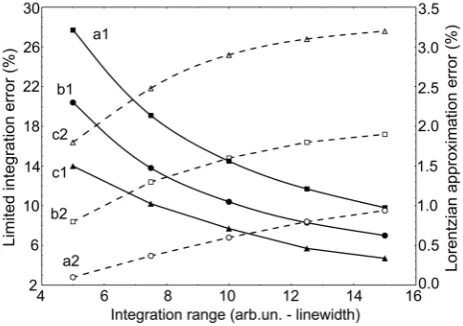
within infinite limits of integration. It is the same for any Gaussian broadening in case the number of molecules in unit volume is the same. However, in real noisy conditions the limited integration range can introduce a significant error. For three cases discussed above two types of graphs are shown in Fig.1. These are: 1) The underline area was integrated within several ranges and normalized to the integral calculated within infinite limits, and 2) combined profile was normalized to simulated single Lorentzian line. In this case the Lorentzian linewidth and maximal line intensity were equalized to those of composite multi-line profile. The curves related to type 1 are marked as a1 – c1 (solid lines) and to type 2 as a2 – c2 (broken lines).
Figure 1. The errors of underline area estimation vs range of integration. The solid lines demonstrate ratio of combined line area to integral in infinite limits (left axis). The broken lines show the ratio of combined line area to approximated Lorentzian line area (right axis).
The second problem of experimental limited integration is a correct determination of zero level. In case of relatively wide line the ground level could be specified with an error of several percentages. That results in additional up to 20-25% error in underline area estimation and introduces errors in line maximum and linewidth measurement.
Finally, due to several reasons, namely: the integration of the line within limited range (±10 linewidth); presentation the line as a pure Lorentzian one; experimental errors of ground level specification, in total, up to 20-50% error can be accumulated in gas concentration measurement. This difference means that, for example, at real 15% concentration of oxygen, the sensor can report 21%. This is absolutely not acceptable from the human life conditions point of view.
3. Interrupted Absorption
In the signal analysis theory the model of interrupted absorption qualitatively explains the line broadening mechanism [41,44]. However, the crucial role in signal spectrum formation plays not only duration of a single pulse but a slope rate at front and back of the pulse. Actually, there
[image:6.595.320.547.175.281.2]is no evidence what is a shape of a real edge of the wave train. It is intuitively clear that the rectangular edge requires infinitely wide spectrum, hence it should be somehow smooth. Let us compare the bell-like (Fig.2, curve 1) and step-like (Fig.2, curve 2) signals with the same width and the step signals of different durations (2-4) but with the same front/back slope rate (optical frequency is not shown).
[image:6.595.62.294.245.408.2]Figure 2. Gaussian (1) and step (2) signals of the same width; shorter step signal (3) and longer one (4). The 3,2,4 pulse duration ratio is approximately like 0.4/1/5.
Figure 3. Spectral distributions of the pulsed signals (1) to (4) shown in Fig.2. The “zero” frequency value corresponds to optical carrying frequency.
The Fourier transformation (Fig.3) confirms well known fact that the Gaussian in-time signal is presented by Gaussian in-spectrum signal. However, the step signal of the same duration has much richer and, in total, wider spectrum. With increase of the step-signal duration (curve 4) the spectral central peak becomes narrower and can achieve linewidth even smaller than that for the Gaussian signal (curve 1).
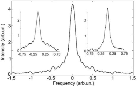
[image:6.595.316.546.332.442.2]were occasionally generated during the data acquisition time. The example of six combined spectra is shown in Fig.4. The insertions show the experimental line profiles averaged through randomly taken consequent six scans.
[image:7.595.57.289.301.446.2]It is evidently that a total spectral underline area is proportional to a total number of absorbing molecules. Since the spectral satellites contain some notable energy, they must be taken into account when gas concentration is being estimated. The satellites can contain from 30% to 50% of total spectral energy. Hence, the precise measurement of the line wings area is very important. The correct position of the background “zero” level is the problem even in classical experimental spectroscopy [45, 46]. Finally, due to all negative factors mentioned above, the gas concentration can be found with error between approximately 15 to 50%. The main problem in the way of correct measurements is to estimate the contribution into error all mentioned above factors in different and changeable external conditions.
Figure 4. Examples of the final spectra composed from light pulses of different duration: central peak represents summation of six consequent spectra similar to those shown in Fig.3. The insertions show experimental
line profiles averaged through randomly taken six scans within a series. From the comparison of the experimental and theoretical profiles it can be concluded:
1) Both experimental and simulated lines demonstrate the peak, which is sharper than the Lorentzian one.
2) The experimental lines are not repeatable, especially in a bottom part: sometimes they have “skirt” (Fig.4, left insertion) larger than the theoretical profile, sometimes smaller (right insertion). The simulated profile is very conditional since in reality each measurement sample accumulates spectra of occasional set of pulses of different durations and amplitudes.
3) Left wing is not similar to right one, especially if the number of summarized scans is smaller than approximately 15 – 20.
4) The more lines are summarized – the wider final linewidth is generated because of maxima position jitter.
4. Photon/Molecule Ratio and Collision
Probability
To solve some complicated mathematical equations the
theoreticians operate with categories “high pressure”, “low pressure” “high/low active/perturber atoms mass ratio”, etc. Such simplifications make possible to achieve an analytical solution in some limited cases. Here we estimate more in detail the air and laser radiation parameters to understand better which limitations are really actual in spectroscopic sensor case.
In experiments we used the 0.3-mW output diode tunable laser with the beam collimated within approximately 1 mm2 cross-section area. The laser wavelength was near 760 nm. The photon energy at this wavelength is 2.6⋅10-19J. Hence, the photon flux was 1.15⋅1015 photons/sec. With 1 mm2 beam cross-section and 1000 mm space between the laser and detector, the beam volume contains 3.8⋅106 photons in each moment of observation. This volume contains 5.4⋅1018 molecules of oxygen. Hence, potentially each photon, running along 1-m distance can meet 1.42⋅1012 oxygen molecules. However, for some reasons, along this distance only 13 photons from thousand are absorbed and the rest ones are “ignored”. It means that only 5⋅104 photons will be absorbed along 1-m beam path (during 3.3ns of photon time-of-flight). In case the sample acquisition time is 100 ns (30 times 3.3ns) the laser beam interacts with 1.5⋅106 molecules among 5.4⋅1018 available ones.
The gas is represented by a tremendous number of molecules that fly in all directions. However, we can consider just one direction and spread our conclusions for any others. Now imagine that all molecules are under collision synchronization conditions – all collisions happen in the same moment of time when each of 68-nm free-flight paths [47] is passed. The averaged space between the molecules is 3.3nm, so, the free-flight path contains about 20 molecules. Two-molecule diameter is approximately 0.7 nm. It means that the “collision area” covers about 1% of laser beam path and contains 5% of all molecules (1/20). Hence, during photon time-of-flight the 5%-portion of all molecules has chance to collide and this event can take place during 1% of time-of-flight. From this point of view the massive of the colliding molecules potentially capable to interact with the photon is 5⋅10-4 of a total number of molecules located in the laser beam space. These only molecules will demonstrate the collisional broadened shape of absorption lines. In case of air the oxygen and nitrogen molecules have similar atomic weight. Hence, total portion of interacting molecules is approximately 4 times higher than estimated above or 2⋅10-3. If the portion of colliding and in this moment absorbing molecules is so small, the other reason of the line broadening is a static pressure.
the absorption line intensity than the same number of slow moving molecules responsible for relatively narrow lines. Moreover, the O2-O2 colliding pair has as twice larger the absorption cross-section as compared with O2-N2 but mechanically they are almost identical.
5. Impact Energy Distribution
5.1. Maxwellian Distribution of the Molecular Energy The Speed Dependent Voigt Profile has been proposed and intensively investigated in the past [28]. The parameters describing the speed-dependent line shift and width have been formally introduced into the Voigt function. Specific view of these parameters depends on the nature of the collisional interaction. However, due to the mathematical problems the solutions of the equation is possible only for some limited cases, which are out of interest for sensor in-field applications. Some different logic of the collisional line shape simulation is proposed here. The higher kinetic energy of colliding molecules – the closer molecules approach one other, the shorter time of collision, the faster an absorption process can be interrupted, and, finally, the wider the absorption linewidth is. It should be noted that category “energy” automatically includes the “mass” and “speed”. These parameters are not considered separately as in previous works.
It was shown above that at standard atmospheric conditions the contribution from the impact broadened lines into absorption line profile is pretty small. However, at higher pressures this mechanism is dominating. In this section the distribution function of the molecular energy of impact will be found.
The energy per degree of freedom is distributed as a chi-square distribution with one degree of freedom [48]. In this case the Maxwellian distribution is typically written as following:
dE kT
E kT
E A dE E
f( ) = exp
−
p (1)
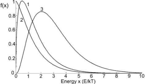
where E is the energy per degree of freedom, k is Boltzmann constant = 0.695 cm-1/K. The coefficient A includes the normalizing constants and parameters, such as T, k,p, and number of molecules in unit volume. At equilibrium, this distribution will hold true for any number of degrees of freedom. In graphs discussed in this paper the variance x is energy E normalized to kT. The graphical view of f(x) is depicted in Fig.5 (curve 1).
5.2. Distribution of Impact Energy
The probability to meet a molecule with energy xi is fi(xi);
the probability to meet a molecule with energy xj is fj(xj), and
probability that such molecules meet one other is fi(xi)×fj(xj).
At front collision the energy of impact is a sum of kinetic energies of molecules: xi + xj. In case the molecule catching
up to one other, the energy of impact is a difference of kinetic energies of molecules: xi – xj. For all colliding molecules, the
[image:8.595.315.550.192.328.2]absorption lines will be broadened and will be Lorentzian in shape because the free-flight time is dispersed around the most probable value within each energy group. The final line is a sum of all lines with different values of broadening.
Figure 5. (1) Maxwellian distribution of molecule kinetic energy; (2) distribution of the impact energies for the catching up molecules; and (3) for frontally colliding molecules. Distribution 2 is normalized to f(x) maximum. The graphs in Fig.5 demonstrate distributions of probability to find specific impact energies: for the catching up molecules (2) and for frontally colliding molecules (3). These graphs demonstrate evident fact: because a large number of molecules moving with the most probable speed, a lot of catching up molecules have a small difference in kinetic energies. Hence, the maximum of impact energy function is shifted to zero energy values. It means that this group of molecules has a minimal collisional broadening and will shape a relatively sharp maximum of the final summarized line. These molecules contribute from any part of kinetic energy spectrum.
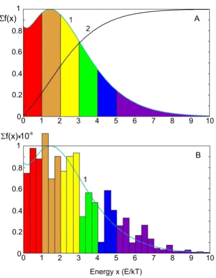
The summarized impact curve has no zero probability at zero energy (Fig.6A). It is approximately the same probability to find the values of molecular collision energy in relatively wide range: from 0 to 3kT. This range accumulates 70% of all colliding molecules and contributes significant part into final line shape.
Figure 6. (A) Summarized curve of both types of collision energy distributions (1); Integration through all values of collision energy (2). Each color demonstrates portion of molecules within 1kT range. The energies higher than 5kT are combined in one group; (B) Chaotically modulated probability curve (1) in case of short data acquisition time.
What is a probability that in each measurement this area will be filled proportionally to curve (1) to generate the smooth and repeatable absorption line? Practically – zero. The chaotic modulation of the line is a natural process; this is not only an experimental noise. The example of probability diagram in case of short data acquisition time can be depicted as shown in Fig.6B. For illustration purpose each kT energy range in Fig.6A is represented by three bars. The amplitudes of them are chaotically modulated and are new ones for each next sample. The summation of a large number of samples results in smooth curve 1.
6. Quazi-Lorentzian Line Shape
Simulation
The line (2) in Fig.6A represents a portion of molecule with collisional energies in range from 0 to x. For illustration purpose the impact energies are grouped in six series: 1) from 0 to 1 contains approximately 20% of all molecules; 2) from 1 to 2 – 25%; 3) from 2 to 3 – 20%; 4) from 3 to 4 – 15%; 5) from 4 to 5 – 10%; and 6) all energies higher than 5 – 10%. Let us consider the simplest model assuming that a linewidth ∆(x) is proportional to the energy of impact x.
∆(x) = m∆0 (2) Here m = 1,2… is a number of energy group as described
above and ∆0 is an initial linewidth depending on total averaged local field of surrounding molecules. The Lorentzian lines with linewidth of ∆(x) are shown in Fig.7 and marked as 1 to 6. In process of final line simulation the lines amplitudes were taken proportionally to percentage of molecules with specific linewidth in each range of the collision energy: 20% (line 1), 25% (line 2), and so on. The final summarized curve (7) can be approximated by simple Lorentzian line (8) with width of 1.75∆0. In the upper part the line can be approximated pretty well, however some notable difference happens in bottom part.
Figure 7. Combination of lines with different linewidth: (1) through (6). The solid line (7) is a summarized line and a dot line (8) shows the Lorentzian profile with maximum and linewidth equal to those of line (7).
The integration of the summarized line (7) and simulated one (8) in infinity limits results in numbers 1 and 0.815, correspondingly. Hence, if the absorption line is interpreted like a simple Lorentzian one, this results in approximately 18.5% error of concentration measurement. Generally, the line maximum is sharper and the wings are wider and higher as compare with Lorentzian profile. Surprisingly, this rough approximation results in realistic line profile. The experimental line averaged through ten scans demonstrates the same view (see Fig.11D).
Simulation with six groups of lines just demonstrates the principles of line shape formation. The line profile can be calculated with continuous summation of the lines and with specific view of the function describing the interaction between the molecules. This consideration will be done in separate paper.
It was discussed in Sec.2.2 that in real conditions, with noise and presence of other, closely located lines, the limited integration range introduces significant error. It can be found that in case discussed in this section the integration within
±10 linewidth range results in 0.725. This means 27.5% difference between composed line area and single Lorentzian line integrated in infinite limits.
[image:9.595.318.546.219.365.2]randomly chosen lines from Fig.7 have been summarized at each frequency point. The specific groups were chosen by a random number program.
Figure 8. (A)Experimental lines (1 – 8) combined near joint middle point and averaged line a slightly shifted up for better identification; (B) Computer simulation of eight and averaged “as is” line b
The simulation in Fig.8B explains why the experimental lines very often are wider and closer to Lorentzian line than it should be from the consideration in the beginning of this Section (Fig.7). Namely, in each specific scan, the line maximum can be slightly shifted because of strong contribution from specific group of lines, which do not coincide with the most probable peak position. This elementary line maximum jitter makes the final line smoother near the sharp peak but practically does not affect the wide wings. We remind again that such line formation is typical for tunable laser spectroscopy and short data acquisition time.
The technological and principle instabilities result in very wide experimental summarized line (see Fig.11C), the linewidth of which cannot be used for gas concentration measurement. However, dynamical combining of the individual scans at line middle point [1,2] results in excellent repeatable profile (see Fig.8A or Fig.11D). This procedure is very effective only if the monitored spectral range contains just a spectrum of a single gas.
7. Lorentzian Line with Maxwellian
Correction
The treatment of the Lorentzian line shape is based on the assumption that correlation function, which means density of probability “do not collide” for a single molecule is described by p1(t) = exp(−t/tc), where tc means average time
between the collisions [44]. The Fourier transformation of
this function results in Lorentzian profile of the spectrum. The p1(t) function is shown in Fig.9 (curve 1) and Fourier spectrum is depicted in Fig 10A. It is commonly accepted that the ensemble of molecules demonstrates the Lorentzian line because it is summation of the same Lorentzian lines. However, some limitation is ignored in this consideration.
Figure 9. Regular correlation function (1) and corrected ones: the collision waves at tc (2), 2 tc (3), and 3 tc (4) were taken into account.
Even at normal atmospheric pressure the molecules are pretty close. Let us consider a group of molecules that collide and start to absorb in the same moment of time t0. The next
wave of collision happens when time is approaching moment
t0 + tc. The main part of molecules moves with the most
probable speed and pass the averaged free-flight distance during average time tc. Hence, among the molecules that
simultaneously started to absorb, the dominant part collides with other molecules when time is approaching t0 + tc.
It is logically to suppose that this wave of collisions has Gaussian-like shape. It describes chaotically scattered moment of time of the second collision. If to add additional Gaussian-like modulation to the p1(t) function with a peak
located at tc, (Fig.9, curve 2) the new spectrum view will
demonstrate some additional wave on the slope of Lorentzian line profile (Fig.10A), curve 2). The molecules that passed the first wave moment without collision will mostly collide around 2 tc (Fig.9, curve 3) and, finally, at 3 tc
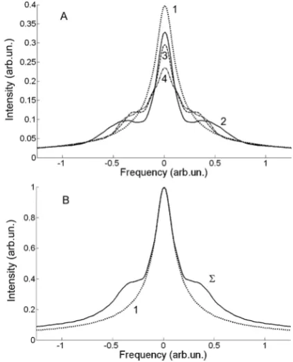
(Fig.9, curve 4). These collision waves result in second and third spectral waves on the Lorentzian profile (Fig.10A). Their positions and amplitudes depend on Gaussian line parameters. The correlation functions have not been normalized in underline areas for better distinguished view of the lines.
A general view of the expression describing the corrected correlation functions can be written as following:
]
)
(
exp
)[
exp(
)
(
23 , 2 ,
1 i
i
i i
C
b
a
t
c
t
t
t
p
=
−
∑
−
−
= (3)
Here ai is a time shift for each collision wave maximum, bi
is Gaussian function width at half maximum, and ci is a
[image:10.595.319.547.161.304.2]correlation functions is the same: fast initial decay and slow delay for big t values. That results in similar relatively narrow central peak (in spectrum) and in wide wings. However, the modulations of a probability function appear as the modulation on the line slopes.
The summation of several types of line results in quite narrow central peak and wide “skirts”. The slight variation of
ai, bi, ci, and tc parameters generates a rich variety of line
[image:11.595.72.284.232.493.2]shapes. It should be noted that summarized profile (Σ) shown in Fig.10B is very similar to the Dicke’s line (narrow peak on the wide pedestal, Fig. 2 in [25]), however, the model used in this consideration is absolutely different.
Figure 10. (A)Spectrum profiles achieved from corrected correlation functions in Fig.9. (B) Lorentzian line (1) and averaged line (Σ) achieved from profiles 2 to 4 in Fig.10A.
8. Data Processing Algorithms
8.1. Consequent Snapshots
In a classical spectrometer each sensor pixel corresponds to a new optical wavelength. The recorded spectrum represents averaged in time radiation of all wavelengths, passing through the entrance slit. In tunable laser spectroscopy the spectral sample is being recorded consequently from “first” to “last” wavelength along a total tunability band. The laser plays role of a light source, slit, and dispersive element. In this case, in each next scan at the same specific wavelength, the sample properties are somehow different because relatively long time is passing between the scans. At fast laser tuning, one registers in a single sample the number of molecules that demonstrate absorption at specific wavelength at this moment of time for
all types of interactions and different linewidth. The fast line scan could demonstrate plateaus, additional local peaks and minima.
The detailed description of the experimental hardware was done in [1,2]. To compare the experimental and theoretical results and to estimate the gas concentration properly, the line profile should be pre-processed to eliminate the noise. However, any data processing modifies somehow the real profile as well. Let us consider first what errors can appear during process of signal averaging.
8.2. Minimally Invasive Algorithms of Data Processing In [1,2] the new algorithms for signal acquisition and processing have been developed. First of all, the sensor estimates the minimal necessary number of scans depending on signal/noise ratio, until the signal achieves trustable parameters. When averaging the spectroscopic signal, not only excess over the noise is important but the positions of the peak and correct shape of the line as well. Any fluctuations of the peak wavelength position may be incorrectly interpreted by the sensor as belonging to another unknown gas; a deformed linewidth results in incorrect estimation of the gas concentration, etc.
Typical averaging algorithm (see, for example, in MS Excel) provides averaging through several consequent points and places the calculated value into the last point of the averaged period. This results in two effects, which are not appropriate from the spectroscopic sensor point of view. Firstly, the line maximum becomes lower and more rounded – the averaging diminishes any spikes: wanted and unwanted. Secondly, the line maximum position moves to the direction of sliding. To somehow avoid this effect in this work we used the symmetrical averaging, when the values from the left and right of the processed point were taking into the calculations. In this case the spectral position of maximum is not changed, however some segments with fast rates are still modified. To minimize this effect, the averaging was performed no more than along ±4 points.
Next practical problem is presence of errors connected with electrical and optical noise. Any noise is some chaotic energy spikes appearing from detector internal noise, surrounding radiation, induction from engines, robot telemetric and radio communication signals, etc. Hence, the averaging makes the signal profile smoother but higher than it really is. The averaging through a relatively small spectral range results in jitter of the background level and, in turn, in errors of the underline area estimation, line intensity and linewidth measurement.
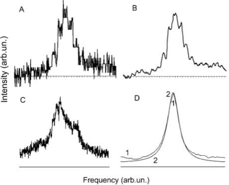
summation is shown in Fig.11D. This profile was compared with the Lorentzian line that was equalized to the same width and maximum (curve 2). As it was discussed in Sec.6 the line maximum is sharper and the wings are wider and higher as compare with Lorentzian profile.
Figure 11. Experimental absorption lines: (A) recorded “as is” single scan; (B) the same scan averaged over 8 points; (C) “as is” summation of 4-scan series, starting from the same pixel number of each scan; (D) averaged line profile (1) through ten scans with floating middle point. Line 2 demonstrates the Lorentzian profile equalized with experimental line at maximum and at the linewidth.
The absorption line position (on the diode current modulation slope) fluctuates or may continuously drift during the measurements because of thermal, electrical current, and mechanical instabilities. As a result, summarizing slightly shifted peaks generates a line profile that is much wider comparing to a normal single line (Fig.11C). This introduces a significant error into the concentration measurements. The summation of several hundred scans that should theoretically improve the signal/noise ratio, results, on the contrary, in a complete disappearance of the signal if the floating point algorithm is not applied.
9. Summary of Errors
The main reasons of measurement errors are uncertainty of a signal ground level position, difference between multi-line composite line profile and Voigt approximation, integration of the line within limited range, and accuracy of the linewidth evaluation in real experimental conditions. For spectral gas sensor operating in atmosphere conditions several reasons of errors could be pointed out:
• The use of Lorentzian approximation instead of Voigt one – 8 -15%
• Limited line area integration (±10 linewidth) – approximately up to 25%
• Model of interrupted absorption: line integration without satellites – 30 - 50%
• Accuracy of line ground level evaluation – 25 - 100%
• Disregarding multi-width line approximation – 25 - 30%
• Processing the spectrum without floating line middle point – up to 100%
• Not taking into account hyperbolized contribution into a line profile from fast molecules – up to 30%
These numbers are approximate and depend on real experimental conditions. However, it is clear that in some situations the final error can overcome hundred percentages.
10. Conclusions
This paper discusses a spectroscopic gas sensor concept with analysis of factors affected the system accuracy. Three groups of problems have been considered:
• Why commonly accepted theoretical approximations can not be used to provide portable sensor high accuracy?
• How to simulate a real line shape maximally fast and effectively?
• What are the typical limitations and/or errors in data processing algorithms?
It was shown theoretically and experimentally that at fast data acquisition, small laser beam cross-section, and short laser beam paths, the absorption line achieved with tunable diode laser is non-repeatable and chaotically modulated in principle, even after averaging of the optical noise. Typically the line is sharper at peak (Super-Lorentzian) and wider at wings (Sub-Lorentzian) as compare with classical profile. In total, three reasons of such line shape have been analyzed in this paper: 1) combination of the lines with different widths achieved from absorbing molecules colliding at different kinetic energy; 2) appearance of the spectral satellites when the absorption process is interrupted in moment of registration; 3) spectral presentation of the correlation function that is modulated by massive molecule collisions at free-flight termination. The natural averaging factors, namely: long optical path, large beam cross section, long acquisition time, and big number of scans result in more repeatable and smooth line profile close to the Voigt shape.
At standard atmospheric conditions the number of oxygen molecules contributing into “collisional width” is negligible as compare with a number of molecules generating the lines with “pressure width”. The fast molecules contribute into the line intensity more than the slow ones.
The general fast algorithm of data processing supposes the approximation of the line shape with Lorentzian profile and correction of the underline area value accordingly to the supplementary data received from independent sensors of pressure, temperature and humidity.
To improve accuracy, reliability, and robotic system survivability we propose the following steps:
• Use pulsed lasers to improve signal/noise ratio and to increase operational range;
• Develop extremely effective single-frequency lasers with nano-selector [49,50] based on the electro-optical drivers (instead of piezo-drivers), which would be immune to mechanical vibrations.
Acknowledgements
This work has been supported by Ontario Centres of Excellence (Canada) through the grants “Synergistic Photonic Sensory Platform” and “Multifunctional Spectroscopy Laser” that were performed in 2009 – 2013 with the financial support from Engineering Services, Inc. (Toronto, ON) and P&P Optica, Inc. (Waterloo, ON). I appreciate controversial remarks from industrial and academic teams that stimulated me to scrupulously analyze classical theoretical approximations and experimental results and find some new ways to solve the accuracy problems. I hope this paper clearly shows that the remote spectroscopy sensors are neither “absolutely useless” as concluded by the industry engineers, nor “completely investigated” as claimed by the university professors.
REFERENCES
[1] I.Matharoo, I.Peshko, A.Goldenberg. Robotic reconnaissance platform. I. Spectroscopic instruments with rangefinders. Rev. Sci. Instrum. Vol. 82, 113107(15 pages), 2011.
[2] I.Matharoo, I.Peshko. Smart Spectroscopy Sensors: II.Narrow-Band Laser Systems. Opt.Lasers Eng. Vol. 51, 270-277, 2013.
[3] Sacher Lasertechnik. Online available from www.sacher-laser.com
[4] G.Berden, R.Peeters, G.Meijer. Cavity ring-down spectroscopy: Experiments schemes and applications. Int.Rev.Phys.Chem. Vol. 19, No. 4, 565-607, 2000.
[5] D.Lisak, J.T. Hodges, R.Ciuryło. Comparison of semiclassical line-shape models to rovibrational H2O spectra measured by frequency-stabilized cavity ring-down spectroscopy. Phys. Rev. Vol. A73, 012507-1 -13 (13 pages), 2006.
[6] S. Wójtewicz, A.Cygan, P.Masłowski, J.Domysławska, D.Lisak, R.S. Trawiński, R.Ciuryło. Spectral lineshapes of self-broadened P-branch transitions of oxygen B band. J. Quant. Spectrosc. Radiat. Transfer. Vol. 144, 36 – 48, 2014. [7] D.S.Bomse, A.C.Stanton, J.A.Silver. Frequency modulation and wavelength modulation spectroscopies: comparison of experimental methods using a lead-salt diode laser. Appl. Opt. Vol. 31, No. 6, 718-731, 1992.
[8] D.M.Bruce D.T.Cassidy. Detection of oxygen using short-extended-cavity GaAs semiconductor diode laser. Appl.Opt. Vol. 29, 1327-1332, 1990.
[9] P.Werle, F.Slemr, M.Gehtz, C.Brauchle. Quantum-limited FM-spectroscopy with a lead-salt diode laser. Appl.Phys. Vol. B49, 99-108, 1989.
[10] C.B.Carlisle, D.E.Cooper, H.Prier. Quantum noise-limited FM spectroscopy with a lead-salt diode laser. Appl.Opt. Vol. 28, 2567 – 2576, 1989.
[11] Ahmed, Rizwan; Baig, M. Aslam. A comparative study of single and double pulse laser induced breakdown spectroscopy. Journal of Applied Physics. Vol. 106, No 3, 033307, 2009.
[12] I. Peshko, R.Pawluczyk, D.Wick. Synergistic Sensory Platform: Robotic Nurse. J. Low Power Electron. Appl. Vol.3, 114-158, 2013.
[13] A.L Dobryakov, S.A. Kovalenko, A.Weigel, J.L.Pérez-Lustres, J.Lange, A. Müller, N.P.Ernsting. Femtosecond pump/supercontinuum-probe spectroscopy: Optimized setup and signal analysis for single-shot spectral referencing. Rev. Sci. Instrum. Vol. 81, 113106, 2010. [14] S-I Chou, D.S.Baer, R.K.Hanson. Spectral Intensity and
Lineshape Measurements in the First Overtone of HF Using Tunable Diode lasers. J. Mol. Spectrosc. Vol. 195, 123-131, 1999.
[15] S-I.Chou, D.S.Baer, R.K.Hanson. Diode-Laser Measurements of He-, Ar-, and N2-Broadened HF Lineshapes in the First Overtone Band. J. Mol. Spectrosc. Vol.196, 70-76, 1999.
[16] F.Slemr, G.W.Harris, D.R.Hastie, G.I.Mackay, H.I.Schiff. Measurement of gas phase hydrogen peroxide in air by tunable diode laser absorption spectroscopy. J.Geophys.Res. Vol. 91, 5371-5378, 1986.
[17] R.Phelan, M.Lynch, J.F.Donegan, V.Weldon. Absorption line shift with temperature and pressure: impact on laser-diode-based H2O sensing at 1.393 µm. Appl. Opt. Vol. 42, No. 24, 4968-4974, 2003.
[18] G. Totschnig, M. Lackner, R. Shau, M. Ortsiefer, J. Rosskopf, M-C. Amann F. Winter. 1.8 μm vertical-cavity surface-emitting laser absorption measurements of HCl, H2O and CH4. Meas. Sci. Technol. Vol. 14, 472-478, 2003. [19] M. Lackner, G. Totschnig, F. Winter, M. Ortsiefer, M-C.
Amann, R. Shau, J. Rosskopf. Demonstration of methane spectroscopy using a vertical-cavity surface-emitting laser at 1.68 μm with up to 5 MHz repetition rate. Meas. Sci. Technol. Vol. 14, 101-106, 2003.
[20] W. Hofmann, M-C. Amann. Long-wavelength vertical-cavity surface-emitting lasers for high-speed applications and gas sensing. IET Optoelectron. Vol. 2, 134-142, 2008.
[21] Honeywell products. Zirconia oxygen (O2) sensor KGZ-10, KGZ-12, GMS-10, MF010 Series, Online available from http://www.directindustry.com/prod/honeywell-sensing-cont rol/zirconia-oxygen-o2-sensors-12365-120200.html
[23] Avalon photonics. Online available from http://www.datasheetarchive.com/AVAP-760-datasheet.html [24] A.Fried, D. Richter. Infrared Absorption Spectroscopy. In: D. E. Heard, editor. Analytical Techniques for Atmospheric Measurement. Oxford UK: Blackwell Publishing, Chap.2, Pp. 72-180, 2006.
[25] R.H. Dicke. The Effect of Collisions upon the Doppler Width of Spectral Lines. Phys.Rev. Vol. 89, No. 2, 472-473, 1953. [26] L.Galatry. Simultaneous Effect of Doppler and Foreign Gas
Broadening on Spectral Lines. Phys.Rev. Vol. 122, No. 4, 1218 – 1223, 1961.
[27] S.G.Rautian, I.I.Sobel’man. The Effect of Collision on the Doppler Broadening of Spectral Lines. Soviet Physics Uspekhi. Vol. 9, No. 5, 701-716, 1967.
[28] P.R.Berman. Speed-dependent collisional width and shift parameters in spectral profiles. J. Quant. Spectrosc. Radiat. Transfer. Vol. 12, 1331-1342, 1972.
[29] A. S. Pine. Line shape asymmetries in Ar-broadened HF( V= 1-0) in the Dicke-narrowing regime. J. Chem. Phys. Vol. 101, No. 5, 3444 – 3452, 1994.
[30] A.S. Pine. Collisional Narrowing of HF Fundamental Band Spectral Lines by Neon and Argon. J. Mol. Spectrosc. Vol. 82, 435-448, 1980.
[31] R.Ciuryło. Shapes of pressure- and Doppler-broadened spectral lines in the core and near wings. Phys.Rev. Vol. A58, No. 2, 1029 – 1039, 1998.
[32] D. Robert, P. Joubert, B. Lance. A velocity-memory model for the spectral lineshape from the Doppler to the collision regime. J. Mol. Struct. Vol. 517–518, 393–405, 2000. [33] R. Ciurylo, A.S. Pine, J. Szudy. A generalized
speed-dependent line profile combining soft and hard partially correlated Dicke-narrowing collisions. J. Quant. Spectrosc. Radiat. Transfer. Vol. 68, 257 – 271, 2001. [34] R. Ciuryło, D. A. Shapiro, J. R. Drummond, A. D. May.
Solving the line-shape problem with speed-dependent broadening and shifting and with Dicke narrowing. II. Application. Phys.Rev. Vol. A65, 012502 (8 pages), 2001. [35] J.-F. D’Eu, B. Lemoine, F. Rohart. Infrared HCN Lineshapes
as a Test of Galatry and Speed-Dependent Voigt Profiles. J. Mol. Spectrosc. Vol. 212, 96–110, 2002.
[36] J.-M. Hartmann, H. Tran, N. H. Ngo, X. Landsheere, P. Chelin, Y. Lu, A.-W. Liu, S.-M. Hu, L. Gianfrani, G. Casa, A. Castrillo, M. Lep`ere, Q. Deli`ere, M. Dhyne, and L. Fissiaux Ab initio calculations of the spectral shapes of CO2 isolated lines including non-Voigt effects and comparisons with experiments. Phys.Rev. Vol. A87, 013403- 1 - 11 (11pages), 2013.
[37] J.-M. Hartmann, V. Sironneau, C. Boulet, T. Svensson, J. T. Hodges, and C. T. Xu. Collisional broadening and spectral shapes of absorption lines of free and nanopore-confined O2
gas. Phys.Rev. Vol. A 87, 032510 (10 pages), 2013.
[38] A.D. May, W.-K. Liu, F.R.W. McCourt, R. Ciuryło, J. Sanchez-Fortun Stoker, D. Shapiro, R. Wehr. The impact theory of spectral line shapes: a paradigm shift. Can. J. Phys. Vol. 91, 879–895, 2013.
[39] Ph. Marteau, Ch. Boulet, D. Robert. Finite duration of collisions and vibrational dephasing effects on the Ar broadened HF infrared line shapes: Asymmetric profiles. J. Chem. Phys. Vol. 80, 3632-3639, 1984.
[40] A. Lucchesinia, S. Gozzini. Collisional broadening and shifting of ammonia absorption lines at 790 nm. Eur. Phys. J(D). Vol. 22, 209-215, 2003.
[41] W.Koechner. Energy Transfer Between Radiation and Atomic Transitions. In: Solid-State Laser Engineering. NY, USA, Springer, 6th ed. Chap.1, Pp. 11 – 37, 2006.
[42] L.S. Rothman, I.E. Gordon, Y. Babikov, A. Barbe, D. Chris Benner, P.F. Bernath, M. Birk, L. Bizzocchi, V. Boudon, L.R. Brown, A. Campargue, K. Chance, E.A. Cohen, L.H. Coudert, V.M. Devi, B.J. Drouin, A. Fayt, J.-M. Flaud, R.R. Gamachem, J.J. Harrison, J.-M. Hartmann, C. Hill, J.T. Hodges, D. Jacquemart, A. Jolly, J. Lamouroux, R.J. Le Roy, G. Li, D.A. Long, O.M. Lyulin, C.J. Mackie, S.T. Massie, S. Mikhailenko, H.S.P. Müller, O.V. Naumenko, A.V. Nikitin, J. Orphal, V. Perevalov, A. Perrin, E.R. Polovtseva, C. Richard, M.A.H. Smith, E. Starikova, K. Sung, S. Tashkun, J. Tennyson, G.C. Toon, Vl.G. Tyuterev, G. Wagner. The HITRAN2012 molecular spectroscopic database. J. Quant. Spectrosc. Radiat. Transfer. Vol. 130, 4–50, 2013.
[43] A.Tan, T.X. Zhang, S.T.Wu. Pressure and density of air in mines. Indian J. Radio Space Phys. Vol. 37, 64-67, 2008. [44] O. Svelto. Interaction of Radiation with Atoms and Ions. In:
Principles of Lasers. New York: Springer-Verlag, 4th ed. Chap.2, Pp. 17 – 58, 2008.
[45] R.E.Meredith. A new method for the direct measurement of spectral line strengths and widths. J.Quant.Spectrosc.Radiat. Transfer. Vol. 12, 455-484, 1972.
[46] R.E.Meredith. Strengths and widths in the first overtone band of hydrogen fluoride. J.Quant.Spectrosc.Radiat.Transfer. Vol. 12, 485-503, 1972.
[47] S. Jennings. The mean free path in air. J. Aerosol Sci. Vol. 19, No. 2, 159-166, 1988.
[48] F. Mandl. The Perfect Classical Gas. In: Statistical Physics. UK, Manchester Physics: John Wiley & Sons, 2nd ed. Chap.7, Pp.184 – 203, 2008.
[49] J.Jabczyński J.Firak, I.Peshko. Single-frequency, thin-film tuned, 0.6 W diode-pumped Nd:YVO4 laser. Applied Optics. Vol. 36, No12, 2484-2490, 1997.