Estimation of Total Energy Load of Building Using
Artificial Neural Network
Rajesh Kumar1, RK Aggarwal2,* and J D Sharma1
1Department of Physics, Shoolini University, Bajhol, Solan 173 212 (India)
2Department of Environmental Science, Dr Y S Parmar University of Horticulture & Forestry, Nauni (Solan), 173230 (India)
*Corresponding Author: [email protected]
Copyright © 2013 Horizon Research Publishing All rights reserved.
Abstract
This paper explores total heat load and total carbon emissions of a six storey building by using artificial neural network (ANN). The energy performance in buildings is influenced by many factors such as ambient weather conditions, building structure and characteristics, the operation of sub-level components like lighting and HVAC systems, occupancy and their behavior. This complex situation makes it very difficult to accurately implement the prediction of building energy consumption. The calculated total load was 2.09 million kW per year. ANN application showed that data was best fitted for the regression coefficient of 0.99812 with best validation performance of 1312.5203 in case of total heat load. To meet out this energy demand fuel options are presented along with their cost and carbon emission and necessary measures has been given.Keywords
Artificial neural network, energy requirement, solar heat gain, internal gain, ventilation losses, carbon emission1. Introduction
Himachal Pradesh is located in north India with Latitude 30o 22' 40" N to 33o 12' 40" N, Longitude 75o 45' 55" E to 79o 04' 20" E, height (from mean sea level) 350 meter to 6975 meter and average rainfall 1300 mm. For our study we have taken a building in Solan district which is located between the longitudes 76.42 and 77.20 degree and latitudes 30.05 and 31.15 degree north the elevation of the district ranges from 300 to 3,000 meter above sea level. The winters during six months (October to March) are severe and people use electricity (provided on subsidized rates) and conventional fuels (wood, LPG and coal). The summers during six months (April to September) people use electricity (provided on subsidized rates) to lower down the temperature. These results are burden on already depleting conventional fuels and same time causing emission of CO2 and global warming. The other option to meet out energy requirement is solar
passive technologies. This requires measured data of solar radiation which is not available in the state. This can be estimated by using various models on the basis of sunshine hour or temperature. The mean hourly values of such data for various places in India are available in the handbook [1]. As in statistical methods we have to deal with higher level of mathematics. Due to tough calculations, the probability of error is more. Evaluation, estimation and prediction are often done using statistical packages such as SAS, SPSS, GENST AT etc. Most of these packages are based on conventional algorithms such as the least square method, moving average, time series, curve fitting etc. The performances of these algorithms are not robust enough when the data set becomes very large. This approach is very much time as well as mind consuming. Therefore ANN is much better than these methods. Neural networks have the potential for making better, quicker and more practical predictions than any of the traditional methods. They can be used to predict energy consumption more reliably than traditional simulation models and regression techniques. Artificial Neural Networks are nowadays accepted as an alternative technology offering a way to tackle complex and ill-defined problems. They are not programmed in the traditional way but they are trained using past history data representing the behaviour of a system.
from small spaces to big rooms. Ekici et al. used the same model to predict building heating loads in three buildings [4]. The training and testing datasets were calculated by using the finite difference approach of transient state one-dimensional heat conduction. Olofsson et al. developed a neural network which makes long-term energy demand (the annual heating demand) predictions based on short-term (typically 2–5 weeks) measured data with a high prediction rate for single family buildings [5]. Reference [6] used a back propagation neural network to predict cooling demand in a building. In their work, a global optimization method called modal trimming method was proposed for identifying model parameters. Kreider et al. reported results of a recurrent neural network on hourly energy consumption data to predict building heating and cooling energy needs in the future, knowing only the weather and time stamp [7]. Based on the same recurrent neural network, [8] predicted the cooling load of three office buildings. Reference [9] used neural networks for the prediction of the energy consumption of a passive solar building where mechanical and electrical heating devices are not used. Considering the influence of weather on the energy consumption in different regions a back propagation neural network to predict building’s heating and cooling load in different climate zones represented by heating degree day and cooling degree day [10]. Reference [11] used a neural network to predict energy consumption for office buildings with day-lighting controls in subtropical climates. Neural network can be used to estimate appliance, lighting and space cooling energy consumption and it is also
a good model to estimate the effects of the socio-economic factors on this consumption in the Canadian residential sector [12]. Reference [13] did Short Term Load Forecasting using ANN Technique. Kreider et al. reported results of recurrent neural networks on hourly energy consumption data [7]. Reference [4] predicted building heating loads without considering climatic variables. Reference [14] studied how statistical procedures can improve neural network models in the prediction of hourly energy loads.
2. Method and Material
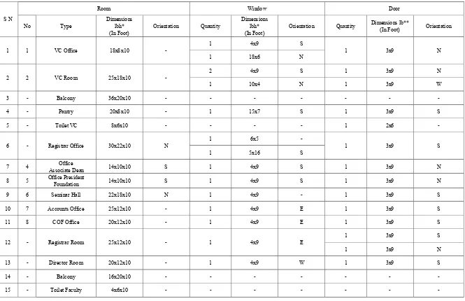
Table 1. Dimensions ofground floor
S N
Room Window Door
No Type Dimensions lbh*
(In Foot) Orientation Quantity
Dimensions lbh*
(In Foot) Orientation Quantity
Dimensions lb**
(In Foot) Orientation
1 1 VC Office 18x8x10 - 1 4x9 S 1 3x9 N
1 18x6 N
2 2 VC Room 25x18x10 - 2 4x9 S 1 3x9 N
1 10x4 N 1 3x9 W
3 - Balcony 36x20x10 - - - -
4 - Pantry 20x8x10 - 1 15x7 S 1 3x9 S
5 - Toilet VC 8x6x10 - - - - 1 2x6 -
6 - Registrar Office 30x22x10 N 1 6x5 - 1 3x9 S
1 5x16 S
7 4 Associate Dean Office 14x10x10 S 1 4x9 S 1 3x9 N
8 5 Office President Foundation 14x10x10 S 1 4x9 S 1 3x9 N
9 6 Seminar Hall 22x18x10 N 1 4x9 - 1 3x9 S
10 7 Accounts Office 25x12x10 - 1 4x9 E 1 3x9 S
11 8 COF Office 20x12x10 - 1 4x9 E 1 3x9 S
12 - Registrar Room 25x12x10 - 1 4x9 E 1 3x9 S
1 3x9 N
13 - Director Room 20x12x10 - 1 4x9 W 1 3x9 S
14 - Balcony 16x20x10 - - - -
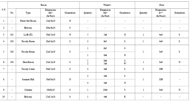
[image:3.808.74.739.97.527.2]Table 2. Dimensions offirst floor
S N
Room Window Door
No Type Dimensions lbh*
(In Foot) Orientation Quantity
Dimensions lbh*
(In Foot) Orientation Quantity
Dimensions lb**
(In Fooot) Orientation
1 - Photo Stat Room 12x10x10 N - - - -
2 - Balcony 20x16x10 S - - - -
3 101 LAB (IT) 50x25x10 N 5 5x6 N 1 4x9 S
4 102 Faculty Room 28x18x10 S 2 6x5 S 1 4x9 S
5 103 Faculty Room 22x12x10 S
1 6x5 S
1 3x9 S
1 8x6 N
6 104 Dean Room 22x12x10 S 1 2 8x6 5x6 W S 1 3x9 N
7 - Faculty Cabin 30x35x10 S 4 4x6 S 2 4X9 -
8 - Seminar Hall 50x30x10 N
2 4x6 S
1 3X9 -
4 4x6 N
9 - Canteen 10x8x10 S 1 10x4 S 1 3x6 N
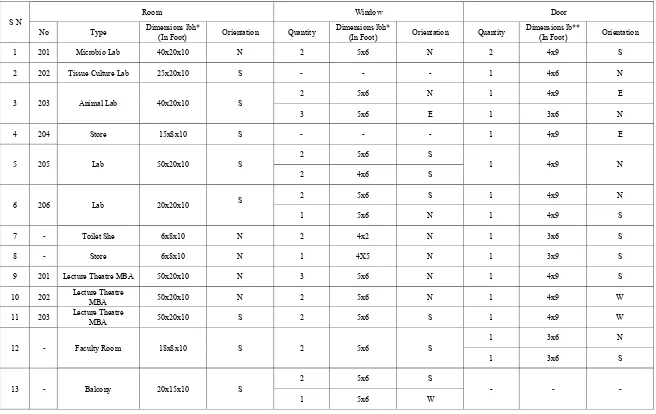
[image:4.808.78.736.84.434.2]Table 3. Dimensions ofsecond floor
S N Room Window Door
No Type Dimensions lbh* (In Foot) Orientation Quantity Dimensions lbh* (In Foot) Orientation Quantity Dimensions lb** (In Foot) Orientation
1 201 Microbio Lab 40x20x10 N 2 5x6 N 2 4x9 S
2 202 Tissue Culture Lab 25x20x10 S - - - 1 4x6 N
3 203 Animal Lab 40x20x10 S 2 5x6 N 1 4x9 E
3 5x6 E 1 3x6 N
4 204 Store 15x8x10 S - - - 1 4x9 E
5 205 Lab 50x20x10 S 2 5x6 S 1 4x9 N
2 4x6 S
6 206 Lab 20x20x10 S 2 5x6 S 1 4x9 N
1 5x6 N 1 4x9 S
7 - Toilet She 6x8x10 N 2 4x2 N 1 3x6 S
8 - Store 6x8x10 N 1 4X5 N 1 3x9 S
9 201 Lecture Theatre MBA 50x20x10 N 3 5x6 N 1 4x9 S
10 202 Lecture Theatre MBA 50x20x10 N 2 5x6 N 1 4x9 W
11 203 Lecture Theatre MBA 50x20x10 S 2 5x6 S 1 4x9 W
12 - Faculty Room 18x8x10 S 2 5x6 S 1 3x6 N
1 3x6 S
13 - Balcony 20x15x10 S 2 5x6 S - - -
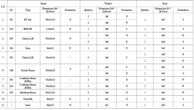
[image:5.808.77.733.124.538.2]Table 4. Dimensions ofthird floor
S N Room Window Door
No Type Dimensions lbh* (In Foot) Orientation Quantity Dimensions lbh* (In Foot) Orientation Quantity Dimensions lb** (In Foot) Orientation
1 301 BT Lab 40x15x10 N
2 5x6 N
1 4x9 S
3 5x6 W
2 302 HOD BT 15x8x10 N 2 4x6 S 1 3x9 S
3 303 Chem LAB 40x20x10 N 2 5x6 N 1 4x6 E
3 5x6 E 1 3x6 S
4 304 Store 6x8x10 N 1 4x5 N 1 3x9 S
5 305 Chem LAB 50x18x10 - 4 5x6 S 1 4x6 N
1 3x6 N
6 306 Faculty Room 20x20x10 S 2 5x6 S 1 4x9 N
1 5x6 N 1 4x9 S
7 301 Confrence Room (MBA) 50x20x10 - 2 5x6 N 1 4x9 W
8 302 Confrence Room (MBA) 50x20x10 - 3 5x6 N 1 4x9 W
9 303 Meditaion Room 40x25x10 3 5x6 N 1 4x9 W
10 - Toilet He 6x8x10 N 2 4x2 N 1 3x6 S
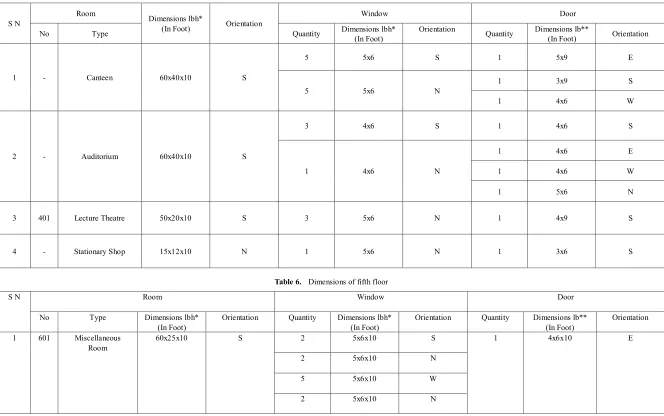
Table 5. Dimensions offourth floor
S N Room Dimensions lbh* (In Foot) Orientation Window Door
No Type Quantity Dimensions lbh* (In Foot) Orientation Quantity Dimensions lb** (In Foot) Orientation
1 - Canteen 60x40x10 S
5 5x6 S 1 5x9 E
5 5x6 N 1 3x9 S
1 4x6 W
2 - Auditorium 60x40x10 S
3 4x6 S 1 4x6 S
1 4x6 N
1 4x6 E
1 4x6 W
1 5x6 N
3 401 Lecture Theatre 50x20x10 S 3 5x6 N 1 4x9 S
[image:7.808.73.737.87.503.2]4 - Stationary Shop 15x12x10 N 1 5x6 N 1 3x6 S
Table 6. Dimensions offifth floor
S N Room Window Door
No Type Dimensions lbh*
(In Foot) Orientation Quantity Dimensions lbh* (In Foot) Orientation Quantity Dimensions lb** (In Foot) Orientation
1 601 Miscellaneous
Room 60x25x10 S 2 5x6x10 S 1 4x6x10 E
2 5x6x10 N
5 5x6x10 W
2 5x6x10 N
Under the steady state approach (which does not account the effect of heat capacity of building materials), the heat balance for room air can be written as given by [15]:
Qtotal = Qc + Qs + Qi + Qv (1) where
Qtotal is total energy requirement if it is –ve then heating is required and if it is +ve then cooling is required.
Qc is conduction losses in a building, Qs is solar gain in a building, Qi is internal gain in a building, Qv is ventilation losses in a building.
2.1 Conduction
The rate of heat conduction (Qc) through any element such as roof, wall or floor under steady state can be written as
Qc = AUΔT (2) where
A = surface area (m2), U = thermal transmittance (W/m2K), ΔT = temperature difference between inside and outside air (K)
If the surface is also exposed to solar radiation then ΔT = Tso - Ti
where Ti is the indoor temperature; Tso is the solar air temperature, calculated using the expression:
Tso = To + αST/ho – εΔR/ho where
To= daily average value of hourly ambient temperature (K), α = absorptance of the surface for solar radiation, ST = daily average value of hourly solar radiation incident on the surface (W/m2)
ho = outside heat transfer coefficient (W/m2K), ε = emissivity of the surface
ΔR = difference between the long wavelength radiation incident on the surface from the sky and the surroundings, and the radiation emitted by a black body at ambient temperature
2.2 Solar Heat Gain
The solar gain through transparent elements can be written as:
Qs = αs Σ AiSgiτi (3) where
αs = mean absorptivity of the space, Ai = area of the ith transparent element (m2), Sgi = daily average value of solar radiation (including the effect ofshading) on the ith transparent element (W/m2), τi = transmissivity of the ith transparent element.
2.3 Ventilation
The heat flow rate due to ventilation of air between the interior of a building and the outside depends on the rate of air exchange. It is given by:
Qv = ρVr CΔT (4) where,
ρ= density of air (kg/m3), Vr = ventilation rate (m3/s), C = specific heat of air (J/kgK)
ΔT = temperature difference (To–Ti) (K)
2.4 Internal Gain
The heat generated by occupants is a heat gain for the building; its magnitude depends on the level of activity of a person.
Qi = (No of people × heat output rate) + Rated wattage of lamps + Appliance load (5) Mean hourly values of data for various places in India are available in the handbook by [1].
Irrespective of developing a new model the neural fitting tool (nftool) of neural network of MATLAB Version 7.11.0.584 (R2010b) with 32-bit (win 32) had been used. Out of six samples four had been used for training, one sample each had been used for validation and testing.
3. Results
The total energy requirement during winter is calculated as (Table 7)
Qm = -1,211,228 kW per annum whose ANN graphs are shown in Fig 1 & Fig 2
The total energy requirement during summer is calculated as (Table 8)
Qm = 874,668 kW per annum whose ANN graphs are shown in Fig 3 & Fig 4
[image:8.595.308.553.555.682.2]Total Load = Heating Load + Cooling Load Total Load = 2,085,896 kW
Table 7. Total heat load in kW [19]
Qc Qs Qv Qi Qtotal
-53.6 90.6 -232.9 78.8 -117.1
Annual
value -2,31,552 1,14,156 -10,06,128 1,51,296 -12,11,228
Table 8. Total cooling load in kW [20]
Qc Qs Qv Qi Qtotal
22.6 67.4 136.1 108.5 334.6
Annual
Figure 1. Validation Performance of Heat load (Qm)
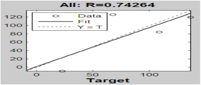
[image:9.595.133.476.134.578.2]Figure 2. Regression Analysis of Heat load (Qm)
Figure 3. Validation Performance of Cooling load (Qm)
[image:9.595.135.477.585.731.2]4. Discussion
In most residential buildings, optimization of thermal comfort and energy consumption is not achieved. From the above system descriptions one can see that ANNs have been applied in a wide range of fields for modeling, prediction and control of building energy systems. What is required for setting up such systems is data that represents the past history and performance of the real system and a suitable selection of ANN models. The accuracy of the selected models is tested with the data of the past history and performance of the real system. The neural network model was used with 10 hidden neurons which didn’t indicate any major problem with the training. The validation and test curves were very similar. The evaluation and validation of an artificial neural network prediction model were based upon one or more selected error metrics. Generally, neural network models which perform a function approximation task will use a continuous error metric such as mean absolute error (MAE), mean squared error (MSE) or root mean squared error (RMSE). The errors will be summed over the validation set of inputs and outputs, and then normalized by the size of the validation set [16]. Here we had used mean squared error (MSE) for the best validation performance. The next step in validating the network was to create a regression plot, which showed the relationship between the outputs of the network and the targets. If the training were perfect, the network outputs and the targets would be exactly equal, but the relationship was rarely perfect in practice. The three axes represented the training, validation and testing data. The dashed line in each axis represented the perfect result – outputs = targets. The solid line represented the best fit linear regression line between outputs and targets. The R value was an indication of the relationship between the outputs and targets. If R = 1, this indicated that there was an exact linear relationship between outputs and targets. If R was close to zero, then there was no linear relationship between outputs and targets.
5. Conclusions
[image:10.595.311.553.79.180.2]The study revealed that the total load of a six storey building is 2.09 million kW thus, heating in winter and cooling in summer is required to meet out this energy demand. If we use electricity it will produce 8.34 ton carbon per annum and the cost of electricity used will be $ 53,776.16 (Table 9). If we use diesel to meet out this energy requirement then 563.19 ton of carbon will be emitted and it will cost $ 139,184.62 [17]. The above results necessitate the use of solar passive technologies to meet out this energy requirement during winters and summers. Increasing awareness of environmental issues has led to development of a large number of energy conservation technologies for buildings, especially in more developed countries [18]. Energy savings potential (ESP) is a very important indicator for developing these technologies.
Table 9. Carbon emission and cost [17]
Fuel Carbon
Emission per kWh (in
g) Total Carbon Emission (in ton) Fuel
Required Total cost (in USD)
Electricity 4 8.34 - 53776.16
Diesel 270 563.19 167302.8 139184.62
Solar
Energy 0 0 0 -
6. Limitations
ANN models like all other approximation techniques have relative advantages and disadvantages. There are no rules as to when this particular technique is more or less suitable for an application. Result of ANN depends upon number of hidden layer neurons. In order to get optimize result we should select optimize number of hidden layer neurons. One way of selecting hidden layer neuron using optimize algorithm technique and other way is hit and trial method. In existing proposed model hit and trial method has been used but it is never easy to comment that the used number of hidden neurons is perfect.
REFERENCES
[1] A. Mani and S. Rangarajan. Solar radiation over India, Allied Publishers, New Delhi, 1982.
[2] S. A. Kalogirou. Artificial neural networks in energy applications in buildings, International Journal of Low-Carbon Technologies, Vol. 1. No. 3, 201–16, 2006. [3] S. A. Kalogirou, C. C. Neocleous and C. N. Schizas.
Building heating load estimation using artificial neural networks, Proceedings of the 17th international conference on parallel architectures and compilation techniques, Toronto, Canada, October, 2008.
[4] B. B. Ekici and U. T. Aksoy. Prediction of building energy consumption by using artificial neural networks, Advances in Engineering Software, Vol. 40, No. 5, 356–62, 2009. [5] T. Olofsson and S. Andersson. Long-term energy demand
predictions based on short-term measured data, Energy and Buildings, Vol. 33, No. 2, 85–91, 2001.
[6] R. Yokoyama, T. Wakui and R. Satake. Prediction of energy demands using neural network with model identification by global optimization, Energy Conversion and Management, Vol. 50, No. 2, 319–27, 2009.
[7] J. F. Kreider, D. E. Claridge, P. Curtiss, R. Dodier, J. S. Haberl and M. Krarti. Building energy use prediction and system identification using recurrent neural networks, Journal of Solar Energy Engineering, Vol. 117, No. 3, 161–6, 1995.
13, 2127–41, 2004.
[9] S. A. Kalogirou and M. Bojic. Artificial neural networks for the prediction of the energy consumption of a passive solar building, Energy, Vol. 25, No. 5, 479–91, 2000.
[10] C. W. Yan and J. Yao. Application of ANN for the prediction of building energy consumption at different climate zones with HDD and CDD, Proceedings of the 2nd international conference on future computer and communication, Wuhan, China, May, 2010.
[11] S. L. Wong, K. K. W. Wan and T. N. T. Lam. Artificial neural networks for energy analysis of office buildings with day lighting, Applied Energy, Vol. 87, No. 2, 551–7, 2010. [12] M. Aydinalp, V. I. Ugursal and A. S. Fung. Modeling of the
appliance, lighting, and space cooling energy consumptions in the residential sector using neural networks, Applied Energy, Vol. 71 No. 2, 87–110, 2002.
[13] S. K. Sheikh and M. G. Unde. Short Term Load Forecasting using ANN Technique, International Journal of Engineering Sciences & Emerging Technologies, Vol. 1, No. 2, 27-107, 2012.
[14] S. Karatasou, M. Santamouris and V. Geros. Modeling and predicting building’s energy use with artificial neural networks: methods and results, Energy and Buildings, Vol. 38, No. 8, 949–58, 2006.
[15] J. K. Nayak and J. A. Prajapati. Handbook on Energy Conscious Buildings, Prepared under the interactive R & D project no. 3/4(03)/99-SEC between Indian Institute of Technology, Bombay and Solar Energy Centre, Ministry of Non-conventional Energy Sources, Government of India, May, 2006.
[16] N. Kartam, I. Flood and J. Garrett. Fundamentals and Applications, ASCE Press, 1996.
[17] Volker Quaschning, Regenerative Energiesysteme, Printed
in Germany, 2011. http://www.volker-quaschning.de/datserv/CO2-spez/index_e
.php
[18] M. Chikada, T. Inou et al. Evaluation of Energy Saving Methods in a Research Institute Building, CCRH. PLEA2001-The 18th Conference on Passive and Low Energy Architecture, Florianopolis-BRAZIL, 883–888, 2001.
[19] Rajesh Kumar, R. K. Aggarwal and J. D. Sharma. Predicting energy requirement for heating the building using artificial neural network, International Journal of Developmental Research, Vol. 3, No. 5, 14-19, 2013.
![Table 7. Total heat load in kW [19]](https://thumb-us.123doks.com/thumbv2/123dok_us/8788869.908323/8.595.308.553.555.682/table-total-heat-load-in-kw.webp)
![Table 9. Carbon emission and cost [17]](https://thumb-us.123doks.com/thumbv2/123dok_us/8788869.908323/10.595.311.553.79.180/table-carbon-emission-cost.webp)
