The Minimum Steiner Tree Problem Based on Genetic Algorithm

(1)

2018 International Conference on Modeling, Simulation and Optimization (MSO 2018) ISBN: 978-1-60595-542-1

The Minimum Steiner Tree Problem Based on Genetic Algorithm

Zhi-hao CHEN

1,*

, Wei-gen HOU

2

and Yun DONG

3

1_{Dept. of Basic Courses, Jiangsu Vocational College of Agriculture and Forestry, Jurong, China}

2_{Dept. of College of Mathematical Science and Engineering, Anhui University}

of Technology, Maanshan, China

3_{Dept. of Teacher Education, Maanshan Teachers College, Maanshan, China}

*Corresponding author

Keywords: Genetic algorithm, Minimum spanning tree, Minimum Steiner tree, Communication network.

Abstract. Genetic Algorithm is a method of searching the optimal solution by using computer to simulate Darwin's biological evolution theory based on natural selection and genetic principles of biological evolution process. This paper aims to solve the problem of the minimum Steiner tree by using genetic algorithm. First, it introduced the concept of genetic algorithm, minimum spanning tree and minimum Steiner tree briefly. Then, it described the application of genetic algorithm in the problem of minimum Steiner tree in detail and gave one method. Finally, this paper has attained the whole approximate root through solving one emulated experimentation emulated about communication network. The solution given in this paper is also applicable to other problems. Its versatility is better. Because of the narrowing of the search range, the search speed is faster and the number of iterations is less.

Introduction

A I (Artificial Intelligence) is known as one of the three most advanced technologies in the world. Evolutionary computation is one of these methods, It includes four typical computing methods: genetic algorithm (GA), genetic programming, evolutionary strategy and evolutionary programming. GA is relatively mature, and is a widely used method at present. It is a computational model that simulates Darwin's natural selection, natural elimination, and survival of the fittest. Genetic algorithms are usually implemented by computer simulation of genetic processes, and often used to search for optimization problems in computational mathematics.[1]

The Minimum Spanning Tree and Minimum Steiner Tree

In a weighted connected graph G( , )V E , if the subgraph 'G contains all the vertices and some

edges in the G and does not form a loop, then the 'G is called the spanning tree of the graph G.

Among them, the spanning tree with minimal weight is called the minimum spanning tree. For solving the minimum spanning tree algorithm is the prim algorithm and Kruskal algorithm which is both the most famous and the most classic algorithm. The latter will be used in this article.If some points can be added in addition to the known vertices, a number of minimum spanning trees can be obtained. And the tree with the smallest total weight in all minimum spanning trees is the minimum steiner tree. The added point is called the steiner point.[2]

Proposition 1 For the known points v v₁, ,...,₂ v_n, the minimum steiner spanning tree always

exists.[3]

Proposition 2 For the known points v v₁, ,...,₂ v_n, assuming that the number of steiner points in the

minimum steiner tree *

(2)

Proposition 3 The ratio of the weights ofthe minimum steiner tree *

T and the minimum spanning

tree T₀ is called the steiner ratio, and the steiner ratio is satisfied

*

0

2 ( )

1

2 ( )

T T

 

  .[5]

Proposition 4 The points P x y₁( , ), ( , ),..., ( , )₁ ₁ P x y₂ ₂ ₂ P x y_n _n _n on the plane is known, assuming

1 2 1 2

max{ , ,..., }, min{ , ,..., },

u n d n

x x x x x x x x

y y y y y y y y

 

then all steiner points are certainly included in the point set {( , )x y x_d  x x y_u, _d  y y_u}.[6] These four propositions indicate:(1)the minimum spanning tree is existent;(2) the number of steiner points is not more than the number of the known points two of the fixed point number minus two;(3) compared with the minimum spanning tree, the route designed with the minimum steiner tree can be reduced by about 13.4% ;(4) the range of coordinate values of steiner points.[7]

The Application of Genetic Algorithm in the Minimum Steiner Tree

The Problem of Wired Communication Network

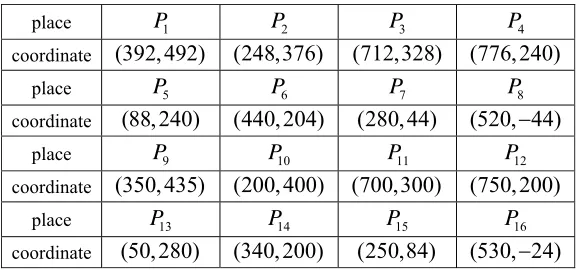
The location of the 16 communication stations on the same level is known. The problem is laying optical cables between these sites and making the least cost. Each location is a vertex of the graph

( , )

G V E .The set of vertices is V { , ,...,P P₁ ₂ P₁₆} .The set of edges is

{ i j, 1, 2,...,16, 1, 2,...,16, }

E PP i j i j . The linear distance between each place is equal to the

[image:2.612.162.450.397.532.2]

weight of the edge.

Table 1. The coordinates of each place (unit: meter).

place P₁ P₂ P₃ P₄

coordinate (392, 492) (248,376) (712,328) (776,240)

place P5 P6 P7 P8

coordinate (88,240) (440,204) (280,44) (520, 44)

place P₉ P₁₀ P₁₁ P₁₂

coordinate (350, 435) (200,400) (700,300) (750,200)

place P₁₃ P₁₄ P₁₅ P₁₆

coordinate (50,280) (340, 200) (250,84) (530, 24)

Because the distance between the two locations is directly proportional to the cost of laying the optical cable, the problem to solve is how to design the laying cable line, making the network connected and the total length of the shortest route.In order to save the cost of laying cables, it is allowed to add s new sites v₁*, *,..., *v₂ v_s outside the known locations, so as to get the smallest

weight tree T*in the graph s V

G , which is the minimum steiner tree problem in practical application.

The Design of Algorithm

Genetic algorithm is an approximate method for solving the minimum steiner tree problem. It consists of 4 main elements: chromosome coding method, individual fitness evaluation, genetic operators and operational factors. In this paper, the genetic algorithm is used to solve t the minimum steiner tree problem. The design of the components is as follows:

(1) Encoding and decoding

(3)

rectangle box, we need to shrink the rectangle area to the square of the unit area with [0,1] [0,1] size, and adjust the corresponding points at the same time.[8]

The binary encoding structure of each individual is as follows:

 









 









 









 









 

absci ssa' s encodi ng ordi nate' s encodi ng absci ssa' s encodi ng ordi nate' sencodi ng



The fi rst poi nt to be sol ved The second poi nt to be sol ved

,



 









 











encodi ng encodi ng



The poi nt to be sol ved absci ssa' s ordi nate' s

,

s

d

here  is 0 or 1.

Each individual is a binary string that is randomly generated, and the length isw_s d_sp.d_s is the

number of Steiner points to be solved, set by yourself when running the program.P is a binary

encoding corresponding to a length of the point to be solved. If it is required to be exact to10k_,then

x y

pd d ,in which d_x _log (10₂ kc_x) ,_ d_y _log (10₂ kc_y)_.

For each individual's decoding, we first need to segment the individual's coding according to the individual structure (such as the upper figure), and then convert every coding to decimal digit.

1 1 2 2

The first point to be solved The second point to be solved _{The point to be solved}

', '

,

',

'

,...,

',

'

s s

s

d d d

x

y

x

y

x

y









then convert the decimal numbers to the point coordinates ( , ), ( , ),...,(x y1 1 x y2 2 xds,yds) ,

' , ' , 1, 2,...,

i x i d i y i d s

x   c x x y  c y y i d ,in which .

In this way, the binary coded individual can be decoded to get all the coordinates of the points to be solved. [9]

(2) Selection of initial group

When the population size is M, according to the required computational accuracy, M binary

strings between 0 and 1 is randomly generated.Then the initial population is constructed.

These M binary strings that do not repeat each other form a single individual. Each individual can

decode the coordinates of the points to be solved according to the (1) method. (3) Evaluation of seeds

For a spanning tree corresponding to an individual, the standard of judging its merits is to see the value of its target function.We take the minimum spanning tree length of the graph with the known points and the points to be solved as the vertex as the target function value. Of course, this value is the smaller the better.[10]

(4) Selection

In this paper, the two methods of wheel selection and optimal preservation strategy are combined to select the individual.

First, the wheel is designed according to the value of the objective function of the individual.Suppose that the objective functions of M individuals are ( ), (T₁₀  T₂₀),..., ( T_M₀). The maximum value is

10 20 0

( *) max{ ( ), (T T T ),..., (T_M )}

     . The difference value is   _i ( *)T ( ),T_i₀ i1, 2,...,M .

Obviously, one of all i must be equal to 0 .

Then the sum of the previous k values is calculated one by one

1

, 1, 2,...,

k k i

i

S  k M





  . Then

calculate the endpoints of each interval

1

, 1, 2,...,

k k M

i i

S

p k M

 

 





.What needs to be pointed out is

1 2

0 p  p  ... p_M 1.

These M endpoints divide the interval [0,1] into M intervals

1

(4)

its target function (Tm0). The length of the M interval is pm pmpm1,(i1, 2,...,M). The length

of the interval directly determines the size of the sector that he occupies on the wheel . The longer the interval, the greater the range it occupies on the wheel; the shorter the interval, the smaller the range it occupies on the wheel.

Then, the number of M numbers r is randomly generated on the interval [0,1]. If r falls within the M interval, the individual that corresponds to it will be retained . The smaller the objective function value

is, the shorter the corresponding interval is, and the smaller the occupied area on the roulette, then the individual is not easy to be selected; otherwise, it is easier to be selected . After repeating this step for many times, individuals with higher fitness will be more likely to be selected and retained.

(5) Hybridization

This paper is a single point cross operation, and the intersection point is randomly generated, and the cross probability is pc 0.03. Two parent individuals exchange strings at random crossover positions to achieve cross operation. All the offspring produced by the cross operation are put into the group, and the parents who have crossed the operation are abandoned.[11]

(6) Mutation

In this paper, one point mutation operation is used, and the mutation probability is 0.03 . The mutation location of the gene is generated randomly, and the number of genes on the gene to perform the mutation from 0 to 1 or from 1 to 0 .[12]

Experimental Analysis and Conclusion

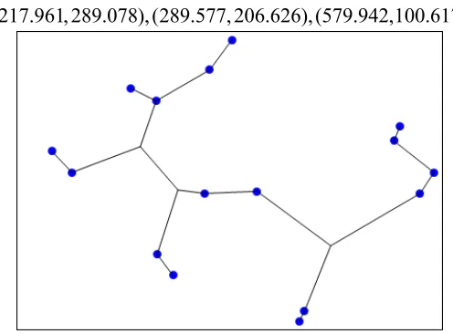
The above solution is programmed through Mathematica11 , and runs through the windows7 system . For the 16 sites given above, we have tested several times that the best effect is when the number of Steiner points is d_s3. By using this method, ten times are solved randomly. And the algorithm can converge to the approximate optimal solution with an average iteration of about 10 times. The optimal approximate solution of the minimum Steiner tree is 1651.854 , while the result of the minimum spanning tree is 1704.7. Compared with the minimum spanning tree, the total path length of the minimum Steiner tree is shortened by 3.1% . The Steiner point is:

[image:4.612.180.428.440.623.2]

(217.961, 289.078),(289.577, 206.626),(579.942,100.617)

Figure 1. The Minimum Steiner tree.

Acknowledgement

(5)

References

[1] Charles Darwin, “The Origin of Species,” Random House, June. 1999, pp. 1-50.

[2] Ying-jie Lei, Shan-wen Zhang and Xu-wu Li, “MATLAB genetic algorithm toolbox and its application,” Xidian University Press, February. 2014, pp. 45-61 (in Chinese).

[3] Kurt Mehlhorn and Peter Sanders “Algorithm and data structure,” Tsinghua University Press, April. 2013, pp. 178 (in Chinese).

[4] Shang-zhi LI, “Course of mathematical modeling competition,” Jiangsu Education Publishing House, June. 1996, pp. 364-385.

[5] Yong-hui Wu and Jian-de Wang, “Algorithm design experiment,” Machinery Industry Press, June.2 013, pp. 399-401(in Chinese).

[6] Courant and Robbins, “What is mathematics,” Oxford University Press, July 1996, pp. 141. [7]D.Z. Du and F.K. Hwang, “A Proof of the Gilbert-Pollak conjecture on Steiner ratio,” Algorithmica, 1992, vol. 1-6, July, pp. 121-135.

[8] Hwang F.K., “An O (n log n)algorithm for rectilinear minimal spanning trees,” Journal of the ACM, 1979, vol. 26(2), February, pp. 177-182.

[9] Bang-yi Liand En-yu Yao, “Shortest path network and its application,” Theory and practice of system engineering, 2000, vol. 6, June, pp. 104-107 (in Chinese).

[10] Douglas S. Reeves and Hussein G. Salama, “A distributed algorithm for delay-constrained unicast routing”, IEEE/ACM Trans on Networking, 2000, vol. 8(2), April, pp. 125-129.

[11] Jiang-wei Li and Lun-hui Xu, “Research on Path Planning Based on Simulated Annealing Algorithm and Neural Network Algorithm,” Automation & Instrumentation, 2017, vol. 32(11), November, pp. 6-31 (in Chinese). DOI: 10.19557/j.cnki.1001-9944.2017.11.002