Scheduling in Distributed Stream Processing Systems
Thesis by
Andrey Khorlin
In Partial Fulllment of the Requirements for the Degree of
Master of Science
California Institute of Technology Pasadena, California
2006
Contents
Acknowledgements 3
Abstract 4
1 Introduction 5
1.1 Background . . . 5
1.2 Streams and Stream Processing . . . 5
1.3 QoS-based Scheduling in Distributed Stream Processing Systems . . . 6
1.4 Formal Problem Denition . . . 7
1.4.1 Server Topology . . . 7
1.4.2 Computation . . . 7
1.4.3 Distributed Scheduling as Optimization over a Queuing Network . . . 8
2 Problem Space and Proposed Scheduling Algorithms 10 2.1 Single Server: Static Mean-Based Scheduling . . . 10
2.1.1 Process Sharing Algorithm . . . 10
2.1.2 Process Sharing Algorithm Model . . . 11
2.1.3 Process Sharing Algorithm Model Approximation . . . 13
2.1.4 Optimum Process Sharing Parameters . . . 16
2.2 Single Server: Dynamic Queue Control Scheduling . . . 16
2.3 Message Reordering . . . 18
2.4 QoS Functions . . . 19
2.5 Cost of Average vs. Average Cost . . . 20
2.6 Distribution of Service Times . . . 21
2.7 Multiple Server Case . . . 22
2.7.1 SMBS . . . 22
2.7.2 DQC . . . 23
3 Theoretical Results 26
3.1 Introduction . . . 26
3.2 Static Sharing Analysis . . . 26
3.3 Optimality of DQC in a Single Server Environment . . . 27
3.4 Scheduling Policies Induced by QoS Functions . . . 28
3.5 Optimality of DQC-NR . . . 29
3.6 Bounds on DQC-NR . . . 31
4 Experimental Results: Single Server 33 4.1 Experimental Settings and Ptolemy . . . 33
4.2 Need for Non-trivial Scheduling . . . 33
4.3 Queue Sizes and Prediction Accuracy . . . 40
4.4 Fast MC Model Approximation Performance Evaluation . . . 41
4.5 Accuracy of Fast Approximation Algorithm . . . 43
4.6 Static Sharing vs. Dynamic Sharing . . . 48
4.7 Cost of Average vs. Average Cost . . . 50
4.8 Smart Scheduling Eectiveness . . . 53
5 Experimental Results: Queuing Network 60
6 Applications 66
7 Related Work 69
8 Future Work 75
9 Conclusions 77
Acknowledgements
I would like to thank Professor K. Mani Chandy for providing me with great help, support and guidance. Through our work on this thesis, I was able to gain a lot of valuable experience. I am also grateful to other members of the Infospheres Lab including Agostino Capponi, Lu Tian, and Daniel Zimmerman for creating a great working environment and providing me with very valuable feedback that helped me in my work on this thesis.
Also, I would like to acknowledge IBM's SMILE Team, including Chitra Dorai, Gerry Buttner, Roman Ginis, Jianren Li, Rob Strom, and Yuanyuan Zhao, with whom I spent a year working as an intern. They provided me with great working experience and exposed me to the area of stream processing, which helped me to arrive at many ideas presented in this thesis.
Last, but not least, I must thank my lovely wife, Olga, for enduring our separation for the past three years and helping us to keep our relationship as strong as the day we got married.
Abstract
Chapter 1
Introduction
1.1 Background
Message-driven or event-driven applications are very well known and used in computer science . The model for such applications is that application components exchange information via sending and receiving messages (or events), which travel along the channels connecting them. This model is very general and is therefore applicable to many practical systems. The model is useful not only for distributed applications, but also in the design of user interfaces, hardware architectures and other domains. In fact, the message-based model describes well the mode of communication among dierent entities in the real world such as departments, companies and people. Thus, any extensions to this model are applicable outside of computer science and distributed systems.
1.2 Streams and Stream Processing
Streaming applications can be viewed as specialized extensions of message-driven applications. In this context, a stream is dened as sequence of messages emitted by a single source with every message having the same schema. Therefore, stream processing is a class of computations that involves receiving one or more streams of messages, executing a program against incoming streams, and producing one or more output streams. The computation can also change, but is assumed to change less frequently than other system parameters. A streaming application is a message-driven application that performs stream processing on several input streams. This denition encompasses many applications. To narrow the denition for the purposes of this discussion, the following key attributes of a streaming application are assumed:
Statefulness: The tasks may have state. This is dierent from ltering or sampling applica-tions that perform computation on one message at a time.
Dynamism:
{ Arrival and service rates for each stream may change rapidly.
{ The number of streams produced and consumed by the application may change at run time.
{ The computation performed by the application may change, but much less frequently than other system attributes.
Performance Requirements: Clients represent performance requirements in the form of Quality of Service (QoS) functions, which dene penalties for the delay incurred in producing output.
Multiple Streams: There may be several streams of information owing through the appli-cations that may or may not share some computation.
Multiple Users: The results are delivered to multiple application users.
Not all stream processing systems exhibit all these features. Only the rst two properties are truly necessary for a system to be a stream processing system. In fact, there are several stream processing systems described in the literature that lack one or more elements of the above list [4].
1.3 QoS-based Scheduling in Distributed Stream Processing
Systems
The requirements described in the previous section put new demands on system design. At the very least, a stream processing system has to process huge numbers of messages while potentially maintaining a large amount of state. Moreover, if the extended requirements for dynamism and performance are necessary, the system must be aware of them too. Since a centralized system is often not capable of meeting such requirements, a distributed implementation of the stream processing system is required. In a distributed stream processing application, computation is broken up into several pieces that are placed onto separate machines.
Parameter Description
S The set of servers in a topology
C The matrix of link capacities between the servers.
Cij = 0 if there is no link between server i and j.
Cij = c > 0 if there is a link with distribution of transmission delays c between server i and j, where i; j 2 [0; jSj]
Note: The matrix is symmetric because links between servers are bidirectional.
Table 1.1: Physical Topology Parameters
allowing each server to converge to an optimal scheduling policy. Thus, we can use the theory of control design to analyze the speed of convergence and stability of our algorithms. We believe that this approach will yield a scheduling algorithm with greater robustness to uncertainty. Similar to Carney et al. [11], we dene a QoS function for each ow, which quanties the cost of delay for every message in every stream. These costs impact the order in which messages should be processed at each server to improve application performance.
1.4 Formal Problem Denition
In this section, we provide a formal denition of the problem. We start by dening server topology and stream computation, and conclude with a denition of scheduling as an optimization problem.
1.4.1 Server Topology
A server topology represents a distributed set of servers that are connected by a set of links. Each server has a certain computational capacity. This capacity is determined by the server's architecture, i.e., CPU speed, cache size, memory size, etc. Similarly, each link has an associated capacity. For the purpose of dening an abstract framework, we use the distribution of service times needed to process each stream's messages to represent the computational capacity of a server. Link capacity is represented as the distribution of time delays for messages traveling on the link (see Table 1.1).
1.4.2 Computation
Parameter Description
F Set of streaming ows where each ow fi is a directed acyclic graph.
fk Single streaming ow dened as a tuple < ~Ck; ~Fk>, where ~Ck is a set
of computations and ~Fk is a connectivity matrix such that ~Fkij = 1 if
~ci2 ~Ck sends output to ~cj2 ~Ck and ~Fkij = 0 otherwise.
m : R2! R Mapping function m(k; i) = j : ~c
i2 ~Ck such that fk2 F is mapped to
server sj 2 S
Yij Set of computations from ow j placed on server i, i.e.,
8~ck2 Yij; ~ck2 ~Cj^ fj 2 F ^ si2 S ^ m(k; i) = j
Table 1.2: Streaming Computation Parameters
Parameter Description
QoS Function q : R ! R maps delay to measure of cost. Measure of cost is comparable
across streams.
Delay computation 8~c; ~c(m1; m2; :::; mn) = m
time stamp( m) = min8i2[0;n](time stamp(mi)) where
time stamp(m) returns time when messages used to generate m or m itself has entered the system.
Table 1.3: Quality of Service Function
therefore we assume that a mapping function, m, is given to us (see Table 1.2). There are several mapping strategies proposed in the literature [6, 55, 59].
1.4.3 Distributed Scheduling as Optimization over a Queuing Network
Now, we dene a notion of quality of service and formulate the distributed scheduling problem as an
optimization problem over a queueing network. Each ow fi2 F is said to have a quality of service
function, q : R ! R. This non-decreasing function maps the delay for every message produced by every ~ck2 ~Ci with ~Fikm = 0; for all m (i.e., each node with zero out-degree).
The delay for each message is computed as follows. Every message entering the system is time-stamped. Each operator in a data ow takes several input messages and produces zero or more messages [1, 4, 29]. An output message carries the highest time-stamp from all messages used to create it. When a nal output message arrives at a sink, the dierence between the current time and the time-stamp is taken. This dierence is called message delay, d, and q(d) is the cost of the delay (see Table 1.3).
metric is minimized. Currently, our optimization metric is dened as the average cost for all ows in the system, where the cost of a ow is dened as the average cost of all messages produced by the ow so far (see Denition 1.4.2).
Denition 1.4.1. Let Qmj be a queue on server si that corresponds to a sub-ow Ymj, and let
[Qm1; :::; Qmn] be a state of all queues on server si, and ! be some feedback information at time t.
Then the scheduling function, sched : (sm; Qm1; :::; Qmn; t; !) ! ~jk, determines which job ~jk2 Qmk should be executed in the next t.
Denition 1.4.2. The Distributed Scheduling Problem is to nd a scheduling function, sched, that
minimizes 1
jF jlimt!1 PjF j
i=0PNitt=0c(dit) Ni
t where N
i
t is the number of events received by stream i before
time t.
Chapter 2
Problem Space and Proposed
Scheduling Algorithms
2.1 Single Server: Static Mean-Based Scheduling
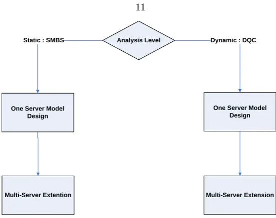
In this chapter, we present two approaches to solve the distributed scheduling problem. The rst approach is a static mean-based scheduling (SMBS) algorithm. The second approach is a dynamic queue-control (DQC) algorithm. We design both approaches in a single server environment and then outline the extensions needed to move these algorithms to a complete queueing network. In addition, we discuss in detail the current assumptions and limitations of both approaches. A summary of our framework is presented in Figure 2.1.
Our rst approach is based on a process sharing algorithm that splits a server's processing capacity among all streams allocated on the server. The process sharing works dynamically such that the capacity is divided among non-idle streams. For this process sharing scheme, we use stream statistics to determine each stream's expected delay under a given share of the total capacity. Then, we use this analysis iteratively to determine the share that minimizes the metric introduced in Section 1.4.3. Since the analysis uses expected queue sizes and delays, we call this approach static mean-based scheduling (SMBS).
2.1.1 Process Sharing Algorithm
At the core of the SMBS approach is the dynamic process sharing algorithm. This algorithm splits the processing capacity needed to execute jobs for each local stream according to the stream's priorities. However, unlike classical static process sharing, which divides the capacity permanently among dierent jobs, the division in this algorithm only occurs when two or more local streams are competing for resources.
The dynamic process sharing algorithm works as follows. For each ow fj on server si there is
Analysis Level
One Server Model Design
One Server Model Design
Multi-Server Extention Multi-Server Extension
[image:12.595.183.460.52.271.2]Static : SMBS Dynamic : DQC
Figure 2.1: Analytical Framework
message reordering is done. The server processes each message until the local stream's computation,
Yij, produces zero or more messages. Therefore, scheduling decisions are not made on a per operator
basis and intermediate results of the computation are not persistent under this scheduling technique, unlike that of Babcock et al. [3]. The scheduling algorithm performs process sharing. Each queue has a priority number assigned to it. If there is more than one non-empty queue, the scheduler gives a share of the local processing capacity based on the priority number of each queue (see Algorithm 1).
Algorithm 1 is executed whenever the current job in stream j nishes processing or a new job
arrives into an empty queue. Later we will see that the priorities fp1; :::; png can be adjusted
to regulate how much of the capacity share each stream should get. This will be at the core of determining a local scheduling policy such that the overall global objective function is minimized. Moreover, we will prove that this mode of sharing is always more ecient than the classical static process sharing scheme in which the shares are not adjusted at run-time. This result is presented in Section 3.2.
2.1.2 Process Sharing Algorithm Model
In order to determine priorities for the process sharing algorithm, we need to understand its behavior. We use queuing theory the same way it is used to derive expected queue sizes for other types of scheduling such as FIFO. We represent our scheduling process as a Markov Chain for which the invariant probabilities are computed. From the invariant probabilities, the expected queue size for each local stream is derived. Then, by application of Little's Law, the average delay is determined.
Algorithm 1 schedule(fQi1; :::; Qing , fmi1; :::; ming , fp1; :::; png,k) Require: 9Qij such that jQijj > 0
Require: 9mij such that mij 6= ;
Require: Pnj=1pj= 1
Require: k 2 [1; n]
Require: fQi1; :::; Qing : set of queues corresponding to local ows
Require: fmi1; :::; ming : set of currently executing jobs
Require: fp1; :::; png : set of priorities
Ensure: Pnj=1~pj= 1
1: if done(mik) then
2: send(mik)
3: end if
4: if size(Qik) > 0 then
5: mik dequeue(Qik)
6: end if
7: for all mij 2 fmi1; :::; ming do
8: totalUsedWeight totalUsedWeight + pj fAggregate shares for all executing jobsg
9: end for
10: for all mij 2 fmi1; :::; ming do 11: p~j totalUsedWeightpj
12: execute(mij, ~pj) fcontinue job execution with given fraction of the CPUg
13: end for
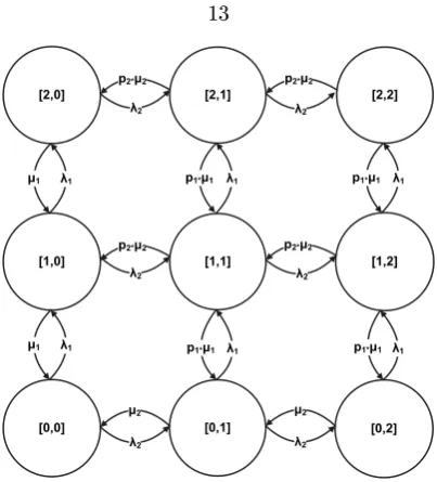
and service rates are distributed exponentially with means jand j respectively. Therefore, we can
construct a continuous Markov chain (CMC) in which each state is a vector of queue sizes for each
local stream Yij (the size of a queue includes the job that is currently being served). An example of
such a Markov chain for two queues with maximum size of two messages is shown in Figure 2.2. The outgoing transitions from each state depend on queue size. If the queue size is zero, then stream share is distributed among the non-empty queues. The following is the denition of the transition function t that determines the rate of transition from state i to state j.
Denition 2.1.1. Given a scheduling algorithm on n queues and given two states Si= [si1; :::; sin]
and Sj = [sj1; :::; sjn], the transition function t : fSi; Sjg ! R species the transition rate from
state Si to state Sj and is dened as
t(Si; Sj) = 8 > > > < > > > :
i if 9sik2 Si; 9sjm2 Sj :: (sjm sik) = 1 ^ 8k 6= k; m 6= m sj m= sik; !ii if 9sik2 Si; 9sjm2 Sj :: (sjm sik) = 1 ^ 8k 6= k; m 6= m sj m= sik;
0 otherwise;
where !i=Pk:sik6=0:pkpi .
Proposition 1. Let M be a continious ergodic Markov chain with transition function t and invariant
distribution . The total residence time for jobs in local ow Yij is
Wi=
P1
j=1siji
[0,0] [1,0]
[2,0] [2,1] [2,2]
[0,1] [0,2]
[1,2] [1,1]
λ1
λ1 λ1 λ1
λ1
λ1
λ2 λ2
λ2 λ2
λ2 λ2
μ1
μ1
p1*μ1
p1*μ1
p1*μ1
p1*μ1
μ2 μ2
p2*μ2 p2*μ2
[image:14.595.223.425.53.276.2]p2*μ2 p2*μ2
Figure 2.2: Example of continuous Markov chain for two queues
Proof. Wi = iqi by Little's Law, where qi is expected queue size. Then, since M is ergodic, qi =
P1
j=1siji.
The Markov chain presented here could be viewed as a multi-dimensional grid of states where the number of dimensions is equal to the number of queues being analyzed. For example, two queues yield a two-dimensional mesh in the rst quadrant, while three queues yield a cube in the rst quadrant. We will use this representation in our further discussion.
2.1.3 Process Sharing Algorithm Model Approximation
Before we can use the abstraction introduced in the previous section, we need to determine a concise way of making predictions with it. Denition 2.1.1 involves an innite Markov chain, which lacks both global and local balance. One way to attack the complexity of the chain is to determine the average amount of sharing that takes place among the streams. If the amount of sharing is known, we can break down the chain into the interior case, when all queues are non-empty, and a set of boundary cases. Then, the model can be disaggregated into subsets that can be analyzed with standard techniques. However, approximating the sharing factor is very complex. The complexity can be illustrated by the case of two streams. We can write down the following equations from the assumption that, in a steady state, the arrival rate equals the service rate:
1= p1b1+ pip11 where p1b = P r(jQi2j = 0 ^ jQi1j > 0), p2b= P r(jQi1j = 0 ^ jQi2j > 0) 2= p2b2+ pip22 where pi= P r(jQi2j > 0 ^ jQi1j > 0)
Now, we have two equations and three unknowns, p1
b, p2b and pi. We cannot use an obvious
third equation, p1
b + p2b+ pi = 1, because it can be derived from the other two equations. A ratio
between interior and boundary probabilities, pi
p1
b+p2b, could be used as a third equation. However,
approximating this ratio is as complex as the original goal.
In the absence of a closed-form solution, we use a numerical approximation of the CMC model. We can approximate the innite chain with a nite chain assuming that queues may not exceed a
certain maximum size, qmax. If qmax is greater than or equal to the true maximum possible size,
then the nite model approximates the innite model perfectly.
Once the model is converted to a nite chain, we can use standard matrix solution to nd invariant probabilities: Q = 0, where Q is the transition matrix [38] (see Denition 2.1.2). However, since Q is singular, we need to perform either equation elimination or equation replacement to nd invariant probabilities. More importantly, matrix Q is very large and its size grows exponentially with the number of queues. For example, with a ve queue model where each queue does not exceed ten
jobs, the total number of cells in Q is (105)2, which clearly cannot t in memory or be processed in
reasonable time.
Denition 2.1.2. (Q-Matrix) Given continuous Markov chain M for scheduling process over fQi1; :::; Qing, where Qij 2 [0; nj], and corresponding transition function t, let projection function
s : R ! Rn project a column or row index of Q to a state Sj2 M:
s(k) = Sj, where Sj = [sj1; :::; sjn] and sjm= R(m)%(nm+ 1)
R(m 1) = R(m)
(nm+ 1)+ sjm , R(n) = k ^ m 2 [1; n]
Dene Q as
Qij= 8 < :
t(s(i); s(j)) if i 6= j;
Prank(Q)
m=1 t(s(i); s(m)) if i = j;
rank(Q) = n Y
i=1 ni
Since direct evaluation of invariant probabilities is not feasible, we present an optimized algo-rithm for nding an approximate invariant distribution. It is based on converting Q into transition probability matrix P , which can be represented concisely using Denition 2.1.2. Thus there is no extra memory needed to look up values of P , since they are obtained by formula evaluation. The invariant probability can be found iteratively (see Algorithm 2):
T
Furthermore, the vector T
t 1 can be represented concisely by rounding numbers in Tt 1 that
are within of zero. The vector is sparse, with non-zero entries occurring in consecutive regions. Therefore, it can be represented as a segment tree that stores information about non-zero segments and allows O(log(jSj) time lookup of entries in , where jSj is the number of segments. Usually, the number of segments is small because the state's probability is centered around the origin.
With concise representations of P and , we perform iteration much faster with much less memory than using a standard matrix approach. The questions of what the initial value of should be and how we determine termination of the algorithm eciently remain. To seed vector we use the following heuristic. From FIFO M/M/1 queue analysis, we know that the probability that the queue has size m is
P r(jQijj = m) = mj (1 j) where j= j
j:
We compute the probability for n up to the maximum size of the queue and then distribute the probability in a uniform fashion among the states whose total queue sizes are the same (see Algorithm 3).
Algorithm 2 predict(P; Niter; ) ! [q1; :::; qn]
1: initialize()
2: [~q1; :::; ~qn] [0; :::; 0] fexpected queue sizes from previous iterationg 3: [q1; :::; qn] [0; :::; 0]
4: iteration 0
5: sum 0
6: while !done([~q1; :::; ~qn]; [q1; :::; qn]; ) ^ iteration < Niter do
7: for all i 2 [1; rank(Q)] do
8: nonZeroEntries getNonZeroIndices(i)
9: for all j 2 nonZeroEntries do
10: if j 6= 0 then
11: ~j= ~j+ jt(i; j)
12: end if
13: end for
14: end for
15: sum t(i;i)1 ~j fweigh next state probability by the holding timeg
16: iteration iteration + 1
17: for all i 2 [1; rank(Q)] do
18: state s(i)
19: normProb t(i;i)sum1j~
20: [~q1; :::; ~qn] [~q1; :::; ~qn] + normProb state
21: end for
22: end while
23: = ~
24: return [q1; :::; qn]
Algorithm 3 initialize() !
Require: f(n; q) ! R; f(n; q) =Pn+1k=1f(k 1; q 1) ^ f(n; 2) = n + 1 : computes total number of
states with total size n over q local queues
1: for i = 0 to n do
2: size Pni=1s(i)
3: i (sizei (1 i))=f(n; q)
4: end for
5: return
In addition, a maximum number of iterations can be set after which termination is mandatory. Both of these termination conditions are used in our approximation algorithm (see Algorithm 4).
Algorithm 4 done([q1; :::; qn]; [~q1; :::; ~qn]; )
1: for i = 0 to n do
2: if jqi ~qij > then
3: return false;
4: end if
5: end for
6: return true
2.1.4 Optimum Process Sharing Parameters
Once we have a scheduling algorithm whose behavior we can predict, we can use this prediction
method to nd the optimal parameters [p1; :::; pn] to minimize the cost of average delay incurred
by each stream. At this point several optimization techniques can be employed. The most general approach based on Genetic Algorithms is utilized to allow the most general family of quality of service functions to be used. The genome is just a set of integers. When they are normalized, they
yield [p1; :::; pn]. The evaluation function is the prediction algorithm that determines average delay
given [p1; :::; pn] (see Algorithms 5 and 6).
Algorithm 5 ndOptimalPartition(N ) ! [p1; :::; pn]
1: population getInitial()
2: for i = 0 to N do
3: population evolve(evaluator)
4: end for
5: [p1; :::; pn] normalize(getFittest(population)) 6: return [p1; :::; pn]
2.2 Single Server: Dynamic Queue Control Scheduling
Algorithm 6 evaluator(P; Niter; ; [p1; :::; pn]) ! cost 1: delay predict(P[p1;:::;pn]; Niter; )
2: cost qi(delay);
3: return cost
can be extended to a distributed multi-server environment. Unlike the algorithm proposed before, this algorithm makes control decisions at every t (for discretized time scale, we assume t = 1). Assuming that there is no cost of switching between tasks, the algorithm selects the most protable piece of work from all available unnished jobs in all queues to be executed in the next t. The algorithm schedules the job whose service rate scaled by the rst derivative of the QoS function at the point equal to the total amount of time spent in the system is the greatest (see Algorithm 7).
Algorithm 7 dynamicQueueControl([mk
1; :::; mkN]) Require: k 2 [0; n] where n is number of local ows
Require: mk
i is a message from local ow k
Require: qk(x) is a QoS function for local ow k
Require: T (mk
i) = time stamp(mki) is time spent in the system since entry
1: maxCost 0
2: j 0
3: for i = 0 to N do
4: marginalCost k dqk(x)dx
x=T (mk i)
5: if marginalCost > maxCost then
6: j i
7: maxCost marginalCost
8: end if
9: end for
10: m~k
j execute(mkj; t) frun job mkj for t units of time; if execute produces output, the job is
done and its results are sent downstreamg
11: if ~mkj 6= ; then
12: end( ~mk
j)
13: end if
This scheduling approach allows messages to be processed out of order. For some streaming applications reordering messages may be infeasible. We discuss the issues of message reordering more in Section 2.3. However, if message reordering is inappropriate, the algorithm can be modied to select only among the messages at the heads of the local queues instead of the total set of all waiting messages. Below, we propose a modied version of Algorithm 7 for the case when message reordering is not permitted. We prove optimality of this algorithm in Section 3.5.
The key modication is the addition of queue size into the metric used to select the next message
for processing. If the message that is going to be processed, mi
1, in the next t nishes, then not
only is the cost of further delay for this message avoided as in Algorithm 7, but the waiting cost for all messages in that queue is also reduced. For each waiting message, the impact of the queue
multiplying it by the number of messages that are in front of each message in the queue. If there is
a model that can predict service time for each message, then the average i 1 can be replaced by
the prediction from the model ~ 1
i .
costRedDueToQueueSize = 0 @Xni
j=1 dqi(x)
dx
x=T (mi j)+ji 1
ni X
j=2 dqi(x)
dx
x=T (mi j)+ji 1
1 A
We call the modied algorithm DQC-NR where "NR" stands for "No Reordering" (see Algorithm 8).
Algorithm 8 dynamicQueueControlNR(si; F; Q; ~Q)
Require: si2 S is a server
Require: F is a set of ows allocated on s
Require: Q is a set of quality of service functions where qi(x) is the QoS function for ow fi2 F
Require: ~Q is a set of queues for each ow fi such that ~qi 2 ~Q : fmi1; :::; minig, where mi1is at the head of the queue
Require: T (mk
i) = time stamp(mki) is time spent in the system since entry
1: maxCost 0
2: j 0
3: for i = 0 to N do
4: costRedDueToQueueSize
P
ni
j=1 dqi(x)dx x=T (mi j)+ji 1
Pni
j=2 dqi(x)dx x=T (mi j)+ji 1
5: marginalCost i
dqi(x)
dx x=T (mi 1)
+ costRedDueToQueueSize
6: if marginalCost > maxCost then
7: j i
8: maxCost marginalCost
9: end if
10: end for
11: m~j1 execute(mj1; t) frun job mj1for t units of time; if execute produces output, the job is
done and its results are sent downstreamg
12: if ~mj16= nil then 13: send( ~mj1)
14: end if
2.3 Message Reordering
Function Name General Form Illustration
Linear cost = a delay + b
Linear Cost Function
0 100 200 300 400 500 600 700
1 1001 2001 3001 4001 5001 6001
Delay (ms) Co s t ( $ )
Concave cost = logb(a delay)
Concave Cost Function
0 0.5 1 1.5 2 2.5 3 3.5 4
1343685 1027 1369 1711 2053 2395 2737 3079 3421 3763 4105 4447 4789 5131 5473 5815 6157
Delay (ms) Co s t ( $ )
Convex cost = delaya
Convex Cost Function
0 50000 100000 150000 200000 250000 300000 350000 400000 450000
1 436 871 1306 1741 2176 2611 3046 3481 3916 4351 4786 5221 5656 6091
Delay (ms) C ost ( $ )
Sigmoid cost = w
1+e(a delayb )
Sigmoid Cost Function
0 20 40 60 80 100 120
1 417 833 1249 1665 2081 2497 2913 3329 3745 4161 4577 4993 5409 5825 6241
[image:20.595.160.490.65.456.2]Delay (ms) C ost ( $ )
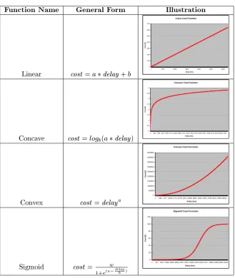
Table 2.1: Types of QoS Functions used
reordering, but DQC performs message reordering depending on the QoS function. We introduced a non-message reordering DQC algorithm. However, it is unclear how to combine DQC and DQC-NR within the same system if only some parts of the system are sensitive to message reordering. In the future, the incorporation of message reordering into the feedback control needs to be studied more extensively. Further issues related to message reordering are discussed by Abadi et al. [1].
2.4 QoS Functions
In the current analysis, four types of Quality of Service functions (linear, concave, convex and sigmoid) are used. The general function forms are presented in Table 2.1.
minimization of the delay for all messages in the stream. The concave function represents the case where only timely messages are valued. The marginal cost of delay diminishes more the longer a message is delayed. The convex function represents streams whose output messages are uniformly valuable. Thus, increasing the delay of any message results in cost blow-up and sti penalties. The sigmoid function is a continuous equivalent of a step function that represents the case when messages with delays up to x are not penalized. However, if a message passes a certain deadline, the penalty becomes substantial.
2.5 Cost of Average vs. Average Cost
In Section 1.3, the SMBS algorithm is described in terms of trying to minimize the cost of average delay. This is dierent from the objective function introduced in Section 1.4.3, which uses average cost instead of cost of average delay. Depending on the quality of service function, this substitution may result in the optimization algorithm being tricked into considering costs that are dierent from the true objective. In this section, the issue of cost of average delay versus average cost of delay is addressed.
For a linear function, it is always the case that both quantities are equal by the property of expected value:
E(cX) = cE(X):
Thus, in case of linear quality of service functions, there is no issue with the SMBS algorithm.
For convex functions delaya, the cost of average will be higher than the average cost. This can
be easily proven for the case when a = 2:
V (X) = E(X2) E(X)2) E(X)2= E(X2) V (X) ) E(X)2 E(X2):
Moreover, the amount by which cost of average overestimates average cost depends on variance, which is determined by our scheduling algorithm. Unfortunately, we have no good model for esti-mating the variance produced by our algorithm.
For concave functions logb(adelay), the cost of average delay underestimates average cost. This
can be intuitively seen from the basic properties of the logarithm:
log(a + b) log(a) + log(b) ) log(a + b) log(ab)
log(E(X)) E(log(X)):
eectively shifts the point of intersection. The point of intersection is important because, near the point of intersection, the change in priorities yields the most eect in terms of the impact on the objective function.
For sigmoid functions the cost of average could either overestimate or underestimate average cost depending on where on the sigmoid QoS curve the average falls. A sigmoid function has the property that the amount of error is bounded by w. However, it also has the most potential for producing erroneous prediction. For example, assume half of the delays yield a cost near zero (in the rst at part of the sigmoid curve) and half of the delays yield a cost near w. Then the average cost could be around w=2. On the other hand, the cost of average delay could be around 0, because average delay falls on the "cheap" part of the QoS curve. This case has the potential to "trick" the optimization algorithm into assuming that giving little or no priority to a stream results in virtually no cost, but in reality the average cost could be quite high.
At this point, we only have a few heuristics that can help the optimization algorithm to yield better predictions. In future work, the relation between average cost and cost of average should be explored more rigorously. Meanwhile, we notice that the distribution of delay under SMBS remains exponential-like. In several experiments the variance change was observed to be roughly similar to
the change of the mean, i.e., if the mean and variance under share p1 are x and v, and the mean
under share p2 is c x, then the variance undre share p2 is c v. This simple heuristic can improve
the optimization portion of our SMBS algorithm. We illustrate these approaches in Section 4.8.
2.6 Distribution of Service Times
2.7 Multiple Server Case
In Section 2.1.1 and 2.2, the queue control algorithms that work in a single server environment were dened. Now, a series of extensions to these algorithms for multiple server environments is discussed. The extensions to the SMBS algorithm are covered rst, followed by discussion of DQC and DQC-NR in multiple server environments.
2.7.1 SMBS
The straightforward way to extend SMBS scheduling is to extend our genetic algorithm approach from Section 2.1.4. The global solution for the whole network can be represented as a two-dimensional
genome of priorities, ~P , where ~Pij is the priority for stream j on server i. Then, the same structure
of the genetic algorithm is used to nd a near optimal partition on each server. The evaluation function for this approach looks at end-to-end delay for each stream induced by all local priorities. The genome with the lowest total cost is the ttest. The system also monitors the mean arrival and service rates of each stream on each server and, when these means change, invokes the algorithm to nd new partitions.
Algorithm 9 globalSMBS(N) ! P
Require: N : Number of evolution iterations
Ensure: 8i , sumni
j=1Pij= 1
1: population getInitial()
2: for i = 0 to N do
3: population evolve(globalEvaluator)
4: end for
5: P getFittest(population)
6: return P
Algorithm 10 globalEvaluator(P; Niter) ! cost
1: cost 0
2: for all fj 2 F do
3: delay 0
4: for all si2 S ^ 9k; m(k; j) = i do
5: delay delay + predict([Pi;1; :::; Pi;ni]; Niter)
6: end for
7: cost cost + qj(delay);
8: end for
9: return cost
Flow 2 Flow 3
Flow 1
0 2 0 4 0 6 0 8 0 1 00 1 2 0
17 5 31 5 052 2 5 73 0093 7 6 14 5 1 35 2 6 56 01 7 0 1 00 2 00 3 00 4 00 5 00 6 00 7 00
11 0012 0013 0014 0015 0016 001 0
1 00 2 00 3 00 4 00 5 00 6 00 7 00
[image:24.595.194.460.60.184.2]11 0012 0013 0014 0015 0016 001
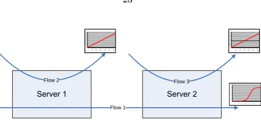
Figure 2.3: Two Server/Three Flow Example
experimental section, cannot eectively be evaluated for more than ve streams on each server. Nonetheless, for small networks, this approach may be sucient and simple enough to use, and for larger networks the presented algorithm can be easily parallelized to provide limited scalability. Alternately, a distributed algorithm could be designed to achieve even better scalability.
2.7.2 DQC
For the dynamic queue control algorithm, the extension to a multiple server environment is complex. The simplest approach is to use DQC and DQC-NR algorithms in a multiple server environment with simple heuristic modications. A complete control algorithm that yields provable, optimal or near-optimal solutions is yet to be developed.
Consider a simple two server/three stream example where just executing a local DQC algorithm without any modications fails to achieve optimality. The mapping of streams to servers is presented below (Figure 2.3).
For simplicity, assume that all three ows have the same arrival and service rates. The quality of service function for each ow is depicted in Figure 2.3. Flow 1 has a sigmoid quality of service
function qi(d) = 10000=(1 + e(20 d=110)), and ows 2 and 3 have linear quality of service function
qi(d) = d. On the rst server, our single server algorithm defers scheduling jobs in ow 1 until the
point where dq1(t)d(t) becomes greater than dq2(t)d(t) , which happens near the inection point where the
derivative of q1(t) starts to grow rapidly. Then, on the second server, the delay for messages in
ow 1 will be at least equal to service time, which causes the total cost to be 10000. If the local algorithm "knew" that delaying messages for ow 1 would result in ultimately higher cost, it would have scheduled these messages ahead of ow 2's messages, even though the metric introduced by Algorithm 7 tells it otherwise.
Now, we introduce a simple extension to our local algorithm that mitigates some of its deciencies.
The extension to Algorithm 7 is simple. We oset the time T (mk
by the expected total service delay. Total service delay is the aggregation of all service times until a local message reaches the user. The new formula for the modied Algorithm 7 computes marginal cost as:
marginalCost = k dqdxk(x)
x=(T (mk i)+!)
where! = Dk X
i=0
ik and Dk is the set of downstream servers on which ow k is located :
The average service time, ij, is tracked on each server for each ow and is fed back upstream
to be used for marginal cost computation.
However, this simple change doesn't work well in all circumstances. True service time experienced on servers downstream may greatly dier from the expected service time. This deviation case is impossible to predict in general. In addition, there is queuing delay downstream, which is even harder to estimate than the deviation from the mean. We explore these issues experimentally in Chapter 4.
2.8 Internet Trac, Flow Intensities and Birth-Death Rates
As mentioned in the introduction, the problem of distributed scheduling and queuing delays is very similar to the rate control problem from the Internet domain. For example, FAST TCP [28] formulates the problem of adjusting the rate of data transmission over the Internet as a control problem and uses well developed control theory tools to prove the stability of a novel TCP algorithm. We are trying to apply a similar approach to streaming systems; these have a more complex structure of data ows than Internet trac because they involve varying service times, ow splits and joins and quality of service functions that assign cost to timeliness of intermediate results rather than utility based on average throughput.
Nonetheless, the study of Internet trac provides valuable insights. The ows on the Internet backbone are usually classied into two groups: long-lived, intensive ows ("elephants") and short-lived, light ows ("mice"). As much as eighty percent of total trac consists of "elephant" ows. Therefore, the analysis in Paganini et al. [39] only looks at long-lived processes. This is important because any control algorithm needs time to react to changes in the system; if changes are fast enough due to a large number of short-lived ows, no control algorithm can react appropriately.
Chapter 3
Theoretical Results
3.1 Introduction
In this chapter, several theoretical results are introduced. Optimality proofs of the DQC and DQC-NR algorithms are presented. In addition, the advantage of the dynamic process sharing scheme used by the SMBS algorithm over the static process sharing scheme is proved.
3.2 Static Sharing Analysis
We start with a proof that the dynamic process sharing algorithm has an advantage over the classical static process sharing algorithm. First, we dene an edge (or boundary) as a set of MC states such that each state has one or more queues empty. For example, such a a set of states for a two queue Markov chain could be all states with the rst queue empty. Second, we dene the static process sharing algorithm. Dynamic process sharing was dened in Section 2.1.1. With these two denitions, we can proove that the dynamic process sharing is superior. The core of the proof is to show that, due to edge states, the static scheme would yield only partial processing capacity to a ow when full capacity is available and there is a temporary state of non-contention.
Denition 3.2.1. Given a continuous Markov process M with state space S, transition rates dened by the dynamic process sharing algorithm from Section 2.1.1, and a set K = f1; : : : ; ng. The edge (or boundary), EK, is a set consisting of all states ~si= fs1; :::sng 2 S such that (8k : k 2 K : sk= 0).
Denition 3.2.2. Given a server s with processing capacity ~Cs, a set of ows F on s where jF j = n,
and a set of priorities fp1; :::; png such that Pni=1pi = 1, the static process sharing scheme is an
algorithm that provisions piC~s to ow fi2 F at all times.
i is the expected service rate and i is the expected arrival rate for ow fi2 F ,
8fi: fi2 F : E(Wfid) < E(Wfis)
where E(Wd
fi) is the expected wait time for ow fi under dynamic process sharing and Wfis is the
expected wait time for ow fi under static process sharing.
Proof. Let K = f1g and P r(EK) be the non-zero probability that all queues except for ow fi are
empty. Without loss of generality, under dynamic sharing, in any state si2 EK, the service rate for
fi under dynamic sharing is i while the service rate under static sharing is pii. Since there exists
time when i > pii, E(qdfi) is less than E(qsfi) where E(qfis) is expected queue size under static
sharing and E(qd
fi) is expected queue size under dynamic sharing. Thus, by Little's Law:
8fi: fi2 F : E(Wfid) < E(Wfis):
The proof depends on the fact that 9KjP r(EK) > 0. This is very easy to show. Let state s0 2 S
such that 8~sj : ~sj 2 s0: ~sj= 0. State s0 corresponds to the case when all queues are empty and no
messages are being processed. The steady state probability for this state is 1 .
P r(s0) = 1 X
8fiinF
fi=fi > 0
Without loss of generality, we also know that the transition probability of moving from state s0 to
state s1= [~s0; :::; ~sn] 2 S such that s1 is a boundary state is
P r(s0! s1) = fi= X
8fiinF
fi> 0:
Therefore, P r(s1) > 0, which shows that there exists K, i.e., K = fjg, for which P r(EK) > 0.
3.3 Optimality of DQC in a Single Server Environment
Now, we prove that the dynamic queue control algorithm minimizes average cost when executed in a single server environment. In this proof, the expected cost of making incremental decisions at each t is determined. Then, the expression that minimizes this expected cost is derived and is shown to be the same as the one used by Algorithm 7.
Theorem 3.3.1. (DQC Optimality Theorem) Given server s and a set of ows F , where each ow
algorithm DQC minimizes the total cost function
1 jF jt!1lim
PjF j i=0
PNi t t=0c(dit) Ni
t
where Ni
t is the number of events received by stream i before time t:
Proof. After t of time, the current job being executed is either nished or needs more time to
nish. The probability that the job nishes in t for stream i is it. Let M be a set of all
unnished jobs at s; then the total cost incurred is the delay for all unprocessed jobs in the queue:
8mk
i : mki 2 M : Cost =
N X
i=1
(dqdxk(x) x=T (mk
i)
t) dqdxk(x) x=T (mk
i) :
Cost is expressed as the summation of the costs for all the jobs minus the cost of the job that actually nishes.
The other case is that the job being executed does not nish. This will happen with probability
1 it. In this case, the total cost of the decision will be
8mk
i : mki 2 M : Cost =
N X
i=1
(dqdxk(x) x=T (mk
i) t):
Thus, the expected cost of processing a job for t of time is
E(Cost) = (it)
N X
i=1
(dqdxk(x) x=T (mk
i)
t) dqdxk(x) x=T (mk
i)
+ (1 it)
N X
i=1
(dqdxk(x) x=T (mk
i) t) E(Cost) = N X i=1
(dqdxk(x) x=T (mk
i)
i dqdxk(x) x=T (mk
i)
t2
Therefore, in order to minimize expected cost, the algorithm DQC has to maximize
i dqdxk(x) x=T (mk
i)
3.4 Scheduling Policies Induced by QoS Functions
convex, concave or sigmoid), DQC degenerates into a well-known scheduling discipline such as rst-come, rst-serve (FCFS), last-rst-come, rst-served (LCFS) or a combination of these two.
Theorem 3.4.1. (QoS-induced Scheduling Disciplines) Given a set of jobs J = fj1; :::; jng, a quality
of service function q, and a scheduling algorithm DQC:
DQC degenerates to FCFS if d2dxq(x) 0
DQC degenerates to LCFS if d2dxq(x) < 0
Proof. Without loss of generality, assume jobs j1; j22 J have arrival times t1and t2, where t1< t2. For the purposes of this proof, we assume that if t1< t2, then the arrival time for j1 is less than for
j2. Moreover, let w be time the job j1 has spent waiting. Then w (t2 t1) is the amount of work
needed for j2. If d 2q(x)
dx 0, then
as w ! 1 , (i dq(x)dx
x=w (t2 t1)) < (i dq(x)
dx
x=w):
Thus j1 will be served before j2, which corresponds to FCFS discipline, because dq(x)dx
x=w! 1 as
w ! 1.
If d2dxq(x) < 0, then
as w ! 1 , (i dq(x)dx
x=w (t2 t1)) > (i dq(x)
dx
x=w):
Thus j2 will be served before j1, which corresponds to LCFS discipline, because dq(x)dx
x=w! 0 as
w ! 1.
Using Theorem 3.4.1, we can conclude that under linear and convex functions DQC degenerates to FCFS, and under a concave function it degenerates to LCFS. Under a sigmoid function, the messages
are served FCFS until the total time in the system reaches the inection point at d2dxq(x) = 0, and
then the messages are served LCFS.
3.5 Optimality of DQC-NR
Now, we show that DQC-NR also achieves optimality if message reordering is not allowed. Generally, the structure of the proof is the same as for DQC. However, an assumption is made that the service time for messages residing in the queue is not known. Expected service time is assumed to be a "good enough" metric of true service time.
Theorem 3.5.1. (DQC-NR Optimality Theorem) Given a server s, a set of ows F where each
queues ~Q where ~qi 2 ~Q corresponds to ow fi 2 F , then scheduling algorithm DQC-NR minimizes the total cost function
1 jF jt!1lim
PjF j i=0
PNi t t=0c(dit) Ni
t ,
where Ni
t is the number of events received by stream i before time t;
under constraint (message reordering prohibited)
G = 8i 2 [0; jF j]; T (mi
k) < T (min) ) Tc(mik) < Tc(min);
where Tc(mik) is the completion time of message mik.
Proof. Similar to Theorem 3.3.1, we dene the marginal cost mc(t) of delaying a message mik for t
of time to be
mc(t0) = dqdxi(x) x=t0
t;
where, as in Theorem 3.3.1, t0= T (mi
1). Dene a function (s; i) as
(s; i) =Xni j=s
mc(T (mij) + ji 1);
where i is an index of the ithow, ni is the total number of messages in ~qiand s is the sth message
from the head in queue ~qi. We note that (1; i) denes the total marginal cost for queue ow fi
and (2; i) denes the total marginal cost for queue ow fi if the rst message completes after t
of time. When we select a message mi
1 at the head of the queue ~qi for processing for the next t
it will nish with probability it and will remain unnished with probability (1 it). If the
message doesn't nish then the total marginal cost for all the queues on this server is
t(i) = n X
j=1 (1; j):
However, if the message nishes, the cost is
t(i) = n X
j=1
(1; j) , where
= mc(T (mi1)) and
= (1; i) (2; i):
queue.
Thus, the expected cost of selecting message mi
1for processing in the next t is
E(Ci) = (1 it)(
n X
j=1
(1; j)) + (it)(
n X
j=1
(1; j) )
E(Ci) =
n X
j=1
(1; j) it
n X
j=1
(1; j) + it
n X
j=1
(1; j) it( + )
E(Ci) =
n X
j=1
(1; j) it( + ):
So, to minimize the expected cost, we need to maximize it( + ). This is what the DQC-NR
algorithm does (see Algorithm 8).
Theorem 3.5.1 shows that Algorithm 8 achieves optimality in the single server environment.
3.6 Bounds on DQC-NR
If message reordering is not allowed, it is interesting to consider how much worse the performance is than when message reordering is permitted. Now, we show the best case and worst case bounds on DQC-NR as compared to DQC. This should provide an intuition about how much is lost by prohibiting message reordering.
Theorem 3.6.1. (Bounds on DQC-NR) Given a server s, a set of ows F with quality of service
functions qi: R ! R, and algorithms DQC and DQC-NR. Let GDQCbe the optimum achieved under
DQC and GDQC NRbe the optimum achieved under DQC-NR. On average,
0 GDQC NR GDQC qi(
jF j X
i=1 qi i);
where qi is the expected queue size for ow i.
Proof. The lower bound can be easily derived from Theorem 3.4.1; given a convex quality of service function, DQC degenerates into FCFS scheduling, which in fact corresponds to DQC-NR. The upper bound can also be derived by using Theorem 3.4.1. We note that, in the worst case, DQC-NR performs FCFS while DQC degenerates into LCFS. Therefore, the message that arrives at the end
Thus, on average the wait time is
W = jF j X
i=1 qi i:
The additional cost incurred is therefore qi(W ) for some ow fi.
Chapter 4
Experimental Results: Single
Server
4.1 Experimental Settings and Ptolemy
This section describes the experimental environment used in our work. All code for the experiments is developed in Java. Whenever experiments are aimed at describing performance of an algorithm, these experiments are performed on IBM ThinkPad T43p with 2 GHz CPU, 1 GB RAM and Sun's
JDK 1.4.206unlessotherwisenoted:
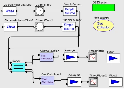
Multi-machine, wide-area experiments are simulated using the Ptolemy discrete event simulator [9] with custom extensions. A discrete event simulation consists of actors that exchange information using messages on a virtual discretized time scale. Ptolemy allows easy addition of custom actors to the simulation engine. In this case, custom actors include servers that implement the described scheduling and control policies (SMBS and DQC), channels that introduce optional delay on message transfer, cost calculators that compute the cost of ultimate delay using provided QoS functions, and data sources that generate messages whose payloads are used to compute simulated service times on each server. Message payloads and interarrival times are distributed exponentially.
An example of a Ptolemy model is shown below for the two streams/ one server example. The links going from data sources to the server and then to cost calculators carry data messages. The links going in the opposite direction carry feedback messages (see Figure 4.1).
We use the simulation as an accurate representation of real-life conditions and utilize simulation results as a baseline for evaluation of our predictive and optimization algorithms.
4.2 Need for Non-trivial Scheduling
SMBS Absolute Advantage
0 500000 1000000 1500000 2000000 2500000 3000000 3500000
0 0.2 0.4 0.6 0.8 1 1.2
Utilization
A
b
s
o
lu
te
A
d
v
a
nt
a
g
e
of
S
M
B
S
ov
e
r FI
FO
Absolute Advantage
Figure 4.2: SMBS vs FIFO on Two Streams with Linear QoS (Absolute Dierence)
Parameters Descriptions
Algorithms SMBS, DQC and DQC-NR
Number of Streams 2
Stream 1 expected interarrival times Between 160 and 4000 Stream 2 expected interarrival times Between 160 and 4000
Stream 1 expected service times 100
Stream 2 expected service times 100
Stream 1 QoS cost = delay
Stream 2 QoS cost = 2000 delay
Table 4.1: Experiment Parameters
As an example of of a nave scheduling policy, a simple FIFO algorithm is chosen. The detailed comparison of SMBS, DQC and DQC-NR against FIFO is performed in Section 4.8.
To show the advantages of smart scheduling, the algorithms are run against FIFO at dierent utilization levels. The parameters for each experiment are listed in Table 4.1. For each algorithm, average cost under linear QoS is generated. The second stream's QoS function weighs delay at 2000 times that of the rst stream. Dierent utilizations are achieved by changing arrival rates for the streams. The average cost is compared to the average cost under FIFO scheduling. The results for all three algorithms are very similar because, under a linear QoS function, all three algorithms degenerate into similar scheduling policies.
DQC Percent Advantage
y = 0.6273x2 + 0.2102x + 0.0133
-20.00% 0.00% 20.00% 40.00% 60.00% 80.00% 100.00%
0 0.2 0.4 0.6 0.8 1 1.2
Utilization P e rc en t A d va n tag e o f D Q C o v er F IF O Percent Difference Trend Line
Figure 4.3: DQC vs. FIFO on Two Streams with Linear QoS (Percent Dierence)
DCQ-NR Absolute Difference
-500000 0 500000 1000000 1500000 2000000 2500000 3000000 3500000
0 0.2 0.4 0.6 0.8 1 1.2
Utilization Ab s o lu te A d v a n ta g e o f DQ C-NR o v e r F IF O Absolute Difference
Figure 4.4: DQC-NR vs. FIFO on Two Streams with Linear QoS (Absolute Dierence)
DQN-NR Percent Difference
y = 0.6117x2 + 0.2239x + 0.0134
-10.00% 0.00% 10.00% 20.00% 30.00% 40.00% 50.00% 60.00% 70.00% 80.00% 90.00% 100.00%
0 0.2 0.4 0.6 0.8 1 1.2
Utilization P e rc e n t Ad v a n ta g e o f DQ C-NR o v e r F IF O Percent Difference Trend Line
SMBC Percent Advantage
y = 0.6065x2
+ 0.2148x + 0.019
0.00% 10.00% 20.00% 30.00% 40.00% 50.00% 60.00% 70.00% 80.00% 90.00% 100.00%
0 0.2 0.4 0.6 0.8 1 1.2
Utilization P e rc e n t A d v a nt a g e of S M B S ov e r F IF O Percent Advantage Trend Line
Figure 4.6: SMBS vs. FIFO on Two Streams with Linear QoS (Percent Dierence)
DQC Absolute Advantage
-500000 0 500000 1000000 1500000 2000000 2500000 3000000 3500000
0 0.2 0.4 0.6 0.8 1 1.2
Utilization A b s o lu te A d v a nt a g e of D Q C ov e r FI FO Absolute Difference
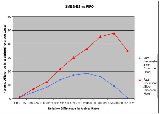
SMBS-ES vs FIFO 0 10 20 30 40 50 60
1.00E-05 0.033592 0.058201 0.111111 0.169591 0.234568 0.388889 0.587302 0.851852
Relative Difference in Arrival Rates
[image:39.595.188.462.73.267.2]P e rcen t D iffe ren ce i n W e ig h ted A v e rag e C o s ts Slow-Inexpensive /Fast-Expensive Flows Fast-Inexpensive /Slow-Expensive Flows
Figure 4.8: SMBS-ES vs. FIFO
In the previous set of experiments, the scheduling algorithms were compared to FIFO. An inter-esting, related question arises from our comparison. Is FIFO equivalent to the fty-fty dynamic process sharing scheme? This question is important for further evaluation of our algorithms. If SMBS with equal shares (SMBS-ES) degenerates to FIFO, it could be used as an alternative base-line for further experiments. To test this hypothesis, FIFO is run against SMBS-ES in a one server, two ows environment with one ow's arrival rate made progressively faster while maintaining the overall utilization at 90% for all runs. Then, the percentage dierence in stream rates is plotted against the dierence in weighted average cost between FIFO and SMBS-ES. This set of experiments is repeated twice, making the fast stream 10 times more expensive than the slow stream and vice versa. The results are depicted in Figure 4.8.
In Figure 4.8, it can be seen that the dierence between FIFO and SMBS-ES grows as the arrival rates diverge. However, if the streams have equal parameters (i.e. arrival and service rates), SMBS-ES does very closely mimic FIFO behavior.
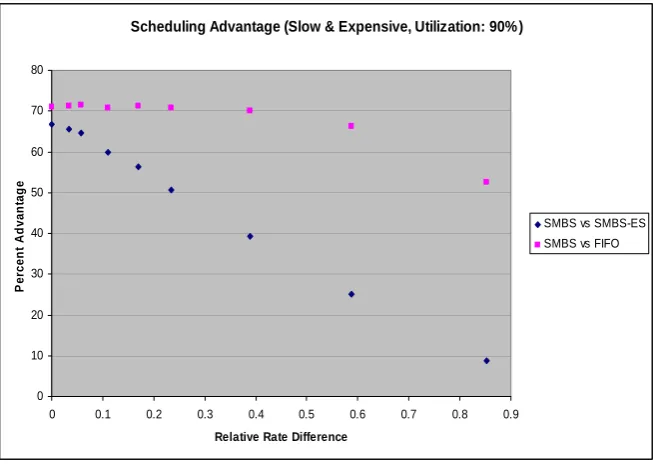
From experiments on SMBS-ES it can be seen that, aside from utilization, the dierence in streams' rates also impacts the ecacy of the smart scheduling algorithms. When there are two streams with one low-cost stream having rare, computationally non-intensive events and the other high-cost stream having frequent, computationally intensive events, changing priorities to prefer the second stream does not change the weighted average cost greatly. In Figures 4.9 and 4.10, the decrease in advantage of SMBS over SMBS-ES and FIFO is shown. The utilization for all the experiments is kept at 90%. The dierence is plotted against relative streams' rate dierence, which
is computed as 1 2
1 . The rest of the parameters are kept the same as in Table 4.1.
Scheduling Advantage (Fast & Expensive, Utilization: 90% )
0 10 20 30 40 50 60 70 80
0 0.1 0.2 0.3 0.4 0.5 0.6 0.7 0.8 0.9
Relative Rate Difference
P
e
rcen
t G
a
in
[image:40.595.157.485.92.324.2]SMBS vs SMBS-ES SMBS vs FIFO
Figure 4.9: Fast Expensive Stream/Slow Inexpensive Stream Advantage Reduction
Scheduling Advantage (Slow & Expensive, Utilization: 90% )
0 10 20 30 40 50 60 70 80
0 0.1 0.2 0.3 0.4 0.5 0.6 0.7 0.8 0.9
Relative Rate Difference
P
e
rc
en
t Ad
v
a
n
tag
e
SMBS vs SMBS-ES SMBS vs FIFO
[image:40.595.158.485.423.655.2]Approximation Error and Matrix Size
0 0.1 0.2 0.3 0.4 0.5 0.6 0.7 0.8 0.9
1 3 5 7 9 11 13 15 17 19 21 23 25 27 29 31 33 35 37 39 41 43
Queue Size (up to maximum queue size)
E
rro
r (
%
)
Experiment 1
Experiment 2
Figure 4.11: Example of Ptolemy Simulation Model
the nave scheduling algorithm even using simple linear QoS functions. Moreover, the most impor-tant fact that aects the amount of improvement is system utilization. On the other hand, the improvement decreases as the dierence in rates between the streams grows.
4.3 Queue Sizes and Prediction Accuracy
We start with a detailed experimental analysis of the SMBS scheduling algorithm. The experiments on the SMBS algorithm are split into a series of steps. First, in this section, the amount of error introduced by substituting the nite Markov Chain for an innite Markov chain is analyzed. Second, the run-time and memory advantages of the fast approximation used by SMBS are shown. Third, the accuracy of the fast approximation is determined. Finally, a comparison among DQC, DQC-NR, SMBS and FIFO is illustrated.
Since our model is based on treating an innite Markov chain as nite, the rst key factor that is important to our approximation is the relationship between the size of the nite chain and the accuracy of the approximation. In other words, we want to know how much accuracy is sacriced when the model size is reduced by assuming that queues do not exceed certain thresholds. The two sets of experiments below answer this question.
Experiment 1 Experiment 2 Steam 1 Steam 2 Steam 1 Steam 2
Mean inter-arrival time 250 250 190 250
Mean service time 100 100 100 70
Priority 1 10 4 7
[image:42.595.239.412.187.252.2]Maximum queue size (from simulation) 44 11 33 13
Table 4.2: Experiment Parameters
State Size Number of Queues
2500 2
15625 3
160000 4
400000 5
Table 4.3: Model Size - Number of Queues Correspondence
approximation becomes accurate quite quickly and, after a queue size of 12 (half of the maximum queue size), the error is within 10%.
4.4 Fast MC Model Approximation Performance Evaluation
Now, we examine the performance of our fast model approximation and compare it to the classical LU decomposition approach on non-sparse matrices and the Conjugate Gradients method (CGS) in conjunction with the Quasi-Minimal Residual method (QMR) on sparse matrices [10, 23]. The experiments are run in the following settings. For LU decomposition, the JAMA matrix package is used [21]. For sparse matrices, a sparse matrix toolkit (SMT) is used [25]. The reason that CGS is used in combination with QMR is that CGS sometimes may not converge to a solution. In this case, QMR is used as a fallback solver. In our experience, such a fallback is rarely needed, while using CGS generally results in faster execution.
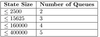
For each experiment, the model is specied as a set of ows with maximum queue sizes, expected service rates, expected arrival rates and relative priorities. The number of states reported in the gure corresponds to the number of states in the Markov chain generated from a model given its specication. Table 4.3 relates the number of states in a chain to number of queues in a model. For each model, the experiment is repeated several times (the standard deviation never exceeds 4% of the mean).
Note: The size of Q is the number of states squared. For example, a 387072 state model results in a 1.49825E+11 cell Q
Run-Time Comparison 0 100 200 300 400 500 600 700 800
169 400 450 900 2025 2500 3375 8000 1562 5062 2E+ 4E+
Number of States in MC
T im e to S o lu ti o n (S ec) LU Solver
Sparce Matrix (CGS/QMR) Fast Model Evalution
Figure 4.12: Run-Time Comparison
Run-Time Comparison (Small Models)
0 1 2 3 4 5 6
169 400 450
Number of States
Ti m e to S o lu ti on (S e c ) LU Solver
Sparse Matrix (QMR/CGS)
Fast Matrix Solver
Figure 4.13: Run-Time Comparison (Small Models)
exponential blowup occurs in much larger models. This fact lets our fast approximation process models dened over 5 queues. In addition, our fast model approximation can be easily parallelized, which would increase its ability to process bigger models (the question of parallelization is deferred to future studies).
An interesting point to be noted is that, for small models, the LU decomposition solver out-performs the CGS/QMR and fast matrix approximation algorithms (see Figure 4.13). This is not surprising, since both algorithms are iteration-based and, on small matrices, LU decomposition per-forms better than iteration-based algorithms. However, the maximum size of matrices for which this is the case is very small, less than 200 states (two queues of maximum 14 messages each).
Memory Used
0 20 40 60 80 100 120
169 400 450 900 2025 2500 3375 8000 1562
5
5062 5
1600 00
3870 72
Model Size (Number of States)
Me
m
o
ry
U
s
e
d
(
M
b
s
)
Fast Matrix Solver
Sparse Matrix (CGS/QMR) LU Solver
Figure 4.14: Memory Comparison
number of states. It is not surprising that the sparse matrix approach performs in between LU decomposition and fast approximation, because it still represents Q explicitly (although in a sparse manner). Moreover, CQS and QSR require some intermediate matrices that increase their memory usage.
In summary, the fast approximation algorithm drastically reduces memory usage and speeds up calculation of steady-state probabilities for large Markov chain models. With the introduction of multi-core processors, by parallelizing fast approximation, the performance could be increased even further. In the next section, the issue of accuracy of the fast approximation algorithm is discussed.
4.5 Accuracy of Fast Approximation Algorithm
We explore how the accuracy of our approximation method depends on various parameters, including
the number of iterations, amount of diusion in the initial vector 0, dierence between streams'
rates, round-o error and number of streams.
We start by looking at the number of iterations. For the purpose of studying the impact of number of iterations, the experiments are run at 90% utilization with two, three and four streams. For each experiment, the number of iterations is increased and the approximation result is compared to the simulation result to determine approximation error. The results are shown in Figure 4.15. Not surprisingly, the approximation becomes more accurate as the number of iterations increases. Also, it can be seen in Figure 4.15 that the more streams there are, the longer it takes to converge to steady-state. The good part is that the dierence in number of iterations between two streams and three streams, and between three streams and four streams, is only two-fold. Thus, the number of iterations does not grow exponentially with the number of streams.
Number of Iterations
-10 0 10 20 30 40 50 60 70 80 90
20 60 100 140 180 220 260 300 340 380 420 460 500 650 850 105
0
Number of Iterations
P
e
rc
e
n
t E
rro
r (
%
)
Two Streams Three Streams Four Streams
Figure 4.15: Number of Iterations and Accuracy of Fast Approximation
and 4.17, the convergence of the two stream approximation is depicted and we can see that the approximation error uctuates at each iteration.
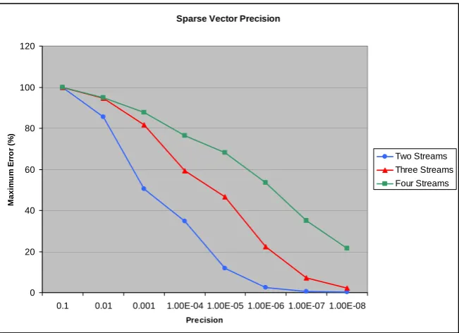
Another parameter that aects accuracy is precision of the sparse vector, . The precision is
a number, , such that for all i < , i is treated as 0. The greater the , the less memory is
needed to store and the greater the approximation error is. To test the impact of precision, the number of iterations is xed while the precision is slowly increased. In Figure 4.18 it can be seen that approximation error decreases as precision increases. Moreover, it is not surprising that the four stream approximation requires higher precision, because of greater probability dispersion.
Figure 4.19 shows the memory savings resulting from decreased precision. By allowing 10% error in the approximation, approximately 50% saving in space is achieved. This rule quanties the benet of rounding.
Now, we examine the impact of dierences in stream rates on approximation error. The same set of experiments on two streams as before is repeated. This time, the arrival rate is varied such that the total utilization is kept constant at 90%. Figure 4.20 depicts approximation error in relation to the dierence in arrival rates. The red line shows the case when the stream with the faster arrival rate is ten times more expensive. The yellow line shows the reverse case. As Figure