2017 2nd International Conference on Computational Modeling, Simulation and Applied Mathematics (CMSAM 2017) ISBN: 978-1-60595-499-8
Research on a Multi-project Scheduling Optimization Algorithm with
Resource Time-Windows
Song-lin LI
*, Xing-ye DONG and Sheng HAN
Beijing Key Lab of Traffic Data Analysis and Mining, School of Computer and Information Technology, Beijing Jiaotong University, Beijing 100044, China
*Corresponding author
Keywords: Multi-project Scheduling Problem, Time-windows, Tabu Search.
Abstract. A resource-constrained multi-project scheduling problem with resource time-windows model is established aimed at minimizing the makespan of multi-project. In terms of solution method, a heuristic algorithm based on Serial Scheduling Generated Scheme is designed to generate an initial solution and a tabu search algorithm is proposed to optimize the solution. Experimental results show that the proposed model is feasible and the proposed method is effective.
Introduction
Project scheduling plays a vital role in organizing work in contemporary enterprises. Issues involving simultaneous management of multiple projects have become more pervasive and acute. According to Payne [1], up to 90% of all projects worldwide are executed in a multi-project environment. Lova et al. [2] who questioned 202 Spanish companies and found that 84% of them run multiple projects in parallel. The resource-constrained multi-project scheduling problem (RCMPSP) is considered as the simultaneous scheduling of two or more projects which demand the same scarce resources. Most prior approaches so far are based on the assumption that resources can be used all the time without considering the possible breakdown. For many actual scheduling problems, it is necessary to take into account time-windows during which some resources such as machines are not available. Scheduling multi-project activities subject to resource time-windows have been rarely considered in the literature over the past few decades. Lambrechts et al. [3] propose the proactive and reactive strategies to solve a new variant of the resource-constrained project scheduling problem (RCPSP), for which the uncertainty is modeled by means of resource availabilities subject to unforeseen breakdowns. Chakrabortty et al. [4] formulate two discrete time-based models to deal with two different disruption scenarios for multi-mode resource constrained problems and propose a reactive re-scheduling procedure to solve the problem. Kreter et al. [5] present three binary linear model formulations that use start-based or changeover-based or execution-based binary decision variables to solve the RCPSP with general temporal constraints and calendars. In this paper, we propose a resource-constrained multi-project scheduling problem with resource time-windows (RCMPSPTW) model which is suitable for solving the possible breakdown of resources and aimed at minimizing the makespan of multi-project. We use the concept of the time-windows to indicate that the fixed resource is in the maintenance state.
The rest of the paper is organized as follows. In Section 2, the RCMPSPTW model is described in detail. Section 3 introduces a heuristic algorithm based on SSGS to generate an initial solution and a tabu search (TS) algorithm to optimize the solution. In Section 4, the computational results and analysis are reported. Finally, the paper is concluded in Section 5.
The Model of RCMPSPTW
Problem Description
Let 𝐽 ≔ {1,2, … , 𝑁𝐽} be the set of jobs, each of which is independent. Each job 𝑖 ∈ 𝐽 consists of a set
𝐽𝑖 ≔ {𝑁𝑖−1+ 1, … , 𝑁𝑖} of real activities as well as a dummy start activity 𝑁𝑖−1+ 1 and a dummy end activity 𝑁𝑖. Activities and precedence constraints of the multi-project are represented by a
finish-to-start activity-on-node (AON) network without time lags. Let 𝐴𝑖𝑗, 𝑖 ∈ 𝐽, 𝑗 ∈ 𝐽𝑖 represent the
activity which is numbered 𝑗 of job 𝑖. The duration of activity 𝐴𝑖𝑗 is described by 𝑑𝑖𝑗. Specifically, for start and end activities of job 𝑖, we have, for all 𝑖 ∈ 𝐽 , that 𝑑𝑖,𝑁𝑖−1+1: = 𝑑𝑖,𝑁𝑖: = 0. Let 𝑆𝑃𝑖, 𝑖 ∈ 𝐽
represent the transfer speed of job 𝑖 when it transfers from one site to another.
Sites are the places where job can only be processed and resources can only be obtained. There are
𝑊 ≔ {1,2, … 𝑁𝑤} types of sites available and the amount of each type is denoted by 𝑤𝑖, 𝑖 ∈ 𝑊. The
set of sites that have mutual exclusion relationships with site 𝑖 is denoted by 𝑀𝐷𝑖 ≔ {𝑗|𝑗 ≠ 𝑖, 𝑖 ∈
𝑤𝑠, 𝑗 ∈ 𝑤𝑠, 𝑠 ∈ 𝑊}, and site 𝑗 ∈ 𝑀𝐷𝑖 indicates that site 𝑖 and site 𝑗 can’t be used simultaneously. Let
𝐷𝑖𝑗 be the distance between site 𝑖 and site 𝑗.
Let 𝐹 ≔ {1,2, … 𝑁𝐹} (𝑀 ≔ {1,2, … 𝑁𝑀}) be the set of fixed resources (move resources) types, and the amount of each type is denoted by 𝐹𝑖, 𝑖 ∈ 𝐹 (𝑀𝑖, 𝑖 ∈ 𝑀). 𝑆𝑃𝑖, 𝑖 ∈ 𝑀𝑘, 𝑘 ∈ 𝑀 represents the transfer speed of move resource 𝑖 when it transfers from one site to another. Moreover, 𝑅𝐴𝐹𝑖𝑗𝑘∈ Ν0
(𝑅𝐴𝑀𝑖𝑗𝑘 ∈ Ν0) represents the amount of fixed (move) resource type 𝑘 ∈ 𝐹 (𝑘 ∈ 𝑀) used constantly by activity 𝐴𝑖𝑗 during an operation phrase. The set of fixed resources that is necessary to carry out
activity 𝐴𝑖𝑗 is denoted by 𝑅𝑖𝑗 ≔ {𝑘|𝑅𝐴𝐹𝑖𝑗𝑘 > 0, 𝑘 ∈ 𝐹}. Specifically, for start and end activities of job
𝑖, we have, for all 𝑖 ∈ 𝐽 , that 𝑅(𝑖,𝑁𝑖−1+1,𝑟)𝐹 : = 𝑅(𝑖,𝑁𝑟,𝑟)𝐹 : = 0, 𝑅(𝑖,𝑁𝑖−1+1,𝑟)𝑀 : = 𝑅(𝑖,𝑁𝑟,𝑟)𝑀 : = 0. In order to
schedule activities subject to break, the time axis [0, 𝑑] is considered, where 𝑑 ∈ Ν0 is the maximum project duration which must not be exceed. Assuming that the time axis is divided into intervals
[0, 1), [1, 2), … [𝑑 − 1, 𝑑), activities may only be started at the beginning of such intervals or at time
𝑑, i.e., at point 𝑡 ∈ 𝑇′ ≔ {0,1, … }. The fixed resource time-windows can be defined as follows: Definition 1. The time-windows for a fixed resource 𝑖 ∈ 𝐹𝑗, 𝑗 ∈ 𝐹 is a step function
𝑇𝑊(∙): [0, 𝑑) → {0,1} continuous from the right at the jump points, where the condition
𝑇𝑊𝑖(𝑡) ≔ {
1, 𝑖𝑓 𝑝𝑒𝑟𝑖𝑜𝑑 [⌊𝑡⌋,⌊𝑡 + 1⌋) 𝑖𝑠 𝑎 𝑤𝑜𝑟𝑘𝑖𝑛𝑔 𝑝𝑒𝑟𝑖𝑜𝑑 𝑓𝑜𝑟 𝑓𝑖𝑥𝑒𝑑 𝑟𝑒𝑠𝑜𝑢𝑟𝑐𝑒 𝑖 0, 𝑖𝑓 𝑝𝑒𝑟𝑖𝑜𝑑 [⌊𝑡⌋,⌊𝑡 + 1⌋) 𝑖𝑠 𝑎 𝑏𝑟𝑒𝑎𝑘 𝑝𝑒𝑟𝑖𝑜𝑑 𝑓𝑜𝑟 𝑓𝑖𝑥𝑒𝑑 𝑟𝑒𝑠𝑜𝑢𝑟𝑐𝑒 𝑖
is satisfied.
Definition 2. Based on fixed resource time-windows, the time-windows 𝑇𝑊𝑖𝑗(𝑡) for activity 𝐴𝑖𝑗
can then be specified by
𝑇𝑊𝑖𝑗(𝑡) ≔ {𝑚𝑖𝑛𝑟∈𝑅𝑖𝑗𝑇𝑊𝑟(𝑡), 𝑖𝑓 𝑅𝑖𝑗 ≠ ∅
0, 𝑜𝑡ℎ𝑒𝑟𝑤𝑖𝑠𝑒
The start (completion) time of activity 𝐴𝑖𝑗 is denoted as 𝑆𝑖𝑗, 𝑖 ∈ 𝐽, 𝑗 ∈ 𝐽𝑖 (𝐶𝑖𝑗, 𝑖 ∈ 𝐽, 𝑗 ∈ 𝐽𝑖). Let
𝑃𝑖𝑗, 𝑖 ∈ 𝐽, 𝑗 ∈ 𝐽𝑖 be the set of all predecessor activities of activity 𝐴𝑖𝑗, 𝑄𝑖𝑗, 𝑖 ∈ 𝐽, 𝑗 ∈ 𝐽𝑖 be the set of
activities that have mutually exclusive relationships with activity 𝐴𝑖𝑗 . Suppose that 𝐴𝑡 ≔ {𝐴𝑖𝑗|𝑆𝑖𝑗 ≤ 𝑡 ≤ 𝐶𝑖𝑗, 𝑖 ∈ 𝐽, 𝑗 ∈ 𝐽𝑖, 𝑡 ∈ 𝑇′} is the set of activities being in operation at time 𝑡. Let
𝐿𝑇𝐽𝑖𝑗, 𝑖 ∈ 𝐽, 𝑗 ∈ 𝑤𝑠, 𝑠 ∈ 𝑊 (𝐿𝑇𝑅𝑖𝑗, 𝑖 ∈ 𝑀𝑘, 𝑘 ∈ 𝑀, 𝑗 ∈ 𝑤𝑠, 𝑠 ∈ 𝑊) represent the time that job 𝑖 (move resource 𝑖) leaves site 𝑗 and let 𝐴𝑇𝐽𝑖𝑗, 𝑖 ∈ 𝐽, 𝑗 ∈ 𝑤𝑠, 𝑠 ∈ 𝑊 (𝐴𝑇𝑅𝑖𝑗, 𝑖 ∈ 𝑀𝑘, 𝑘 ∈ 𝑀, 𝑗 ∈ 𝑤𝑠, 𝑠 ∈ 𝑊) be the time that job 𝑖 (move resource 𝑖) arrives at site 𝑗.
Mathematical Model
The aim of the RCMPSPTW is to find a feasible multi-project schedule S ≔ (𝑆1, 𝑆2, … 𝑆𝑁), in which
𝑆𝑖 ≔ ((𝑠𝑖1, 𝑐𝑖1), (𝑠𝑖2, 𝑐𝑖2), … (𝑠𝑖𝑁𝑖, 𝑐𝑖𝑁𝑖)). In each schedule 𝑆𝑖, the constraints of resource capacities,
min{ max 𝐶𝑖𝑁𝑖, 𝑖 ∈ 𝐽, 𝑁𝑖 ∈ 𝐽𝑖} (1)
s.t: 𝑆𝑖𝑗 ≥ 𝐶𝑖ℎ , ∀ℎ ∈ 𝑃𝑖𝑗, ∀𝑖 ∈ 𝐽, ∀𝑗 ∈ 𝐽𝑖 (2)
𝑆𝑖ℎ ≥ 𝐶𝑖𝑗∨ 𝐶𝑖ℎ ≤ 𝑆𝑖𝑗, ∀ℎ ∈ 𝑄𝑖𝑗, ∀𝑖 ∈ 𝐽, ∀𝑗 ∈ 𝐽𝑖 (3)
𝑆𝑖𝑗 + 𝑑𝑖𝑗 ≥ 𝐶𝑖𝑗, ∀𝑖 ∈ 𝐽, ∀𝑗 ∈ 𝐽𝑖 (4)
𝑆𝑖𝑗, 𝐶𝑖𝑗 ∈ 𝑇′, ∀𝑖 ∈ 𝐽, ∀𝑗 ∈ 𝐽 𝑖 (5)
∑𝐶𝑖𝑗𝑇𝑊𝑖𝑗(𝑡) = 𝑑𝑖𝑗 𝑆𝑖𝑗 , ∀𝑖 ∈ 𝐽, ∀𝑗 ∈ 𝐽𝑖, 𝑡 ∈ 𝑇 ′ (6)
∑𝐴𝑖𝑗∈𝐴𝑡𝑅𝐴𝐹𝑖𝑗𝑟 ≤ 𝐹𝑟, ∀𝑟 ∈ 𝐹, 𝑡 ∈ 𝑇 ′, ∀𝑖 ∈ 𝐽, ∀𝑗 ∈ 𝐽 𝑖 (7)
∑ 𝑅𝐴𝑀𝑖𝑗𝑟 ≤ 𝑀𝑟, ∀𝑟 ∈ 𝑀, 𝑡 ∈ 𝑇′, ∀𝑖 ∈ 𝐽, ∀𝑗 ∈ 𝐽 𝑖 𝐴𝑖𝑗∈𝐴𝑡 (8)
max𝐶𝑖𝐽𝑖 ≤ 𝑑, ∀𝑖 ∈ 𝐽, ∀𝑗 ∈ 𝐽𝑖 (9)
𝐴𝑇𝐽𝑖𝑗 ≥ 𝐿𝑇𝐽𝑖𝑘+ 𝐷𝑗𝑘⁄𝑆𝑃𝑖, ∀𝑖 ∈ 𝐽, {𝑗, 𝑘} ∈ 𝑤𝑠, 𝑠 ∈ 𝑊 (10)
𝐴𝑇𝑅𝑖𝑗 ≥ 𝐿𝑇𝑅𝑖𝑘+ 𝐷𝑗𝑘⁄𝑆𝑃𝑖, ∀𝑖 ∈ 𝑀𝑛, 𝑛 ∈ 𝑀, {𝑗, 𝑘} ∈ 𝑤𝑠, 𝑠 ∈ 𝑊 (11)
The objective (1) is to minimize the makespan of multi-project. Constraint (2) and Constraint (3) represent the precedence constraints and mutual exclusion constraints among activities, respectively. Constraint (4) represents the finish-start precedence relationships among activities. Constraint (5) describes the range of start time and completion time of the activities. Constraint (6) makes sure that the constraints of time-windows are satisfied. Constraint (7) (Constraint (8)) guarantees the given fixed (move) resource capacities are not exceed at any time. Constraint (9) guarantees the maximum completion time of all activities must be completed before the end of the prescribed maximum project duration. Constraint (10) (Constraint (11)) represents that the transfer time of a job (move resource) takes between sites should meet the distance between sites and the transfer speed of the job (move resource).
Solution Procedures
Inspired by Krüger [6], the proposed heuristic algorithm based on SSGS is designed to generate an initial solution for RCMPSPTW and inspired by Mike et al [7], the proposed TS is designed to improve the initial solution.
Notations Definition:
TJ ≔ {𝑖|𝑖 ∈ 𝐽}: the set of jobs who participate in the current task in a scheduling.
TO ≔ {𝑖|𝑖 ∈ {1,2, … |𝑇𝐽|}}: the set of transfer order of jobs.
𝐹𝐺𝑖𝑗𝑘 ≔ {0,1}: the flag which represents the support capability of site 𝑖 for activity 𝐴𝑗𝑘.
𝑇𝐿𝑖 ≔ {𝐴𝑗𝑘|𝑖 ∈ 𝑤𝑠, 𝑠 ∈ 𝑊, 𝑗 ∈ 𝐽, 𝑘 ∈ 𝐽𝑗, 𝐹𝐺𝑖𝑗𝑘: = 1}: the tabu list for site 𝑖.
𝑆𝑔 ≔ {𝐴𝑖𝑗|𝑖 ∈ 𝐽, 𝑗 ∈ 𝐽𝑖, 𝑔 ∈ {1,2, … , |𝐺|}}: the scheduled set, consist of all the activities whose start time, completion time and needed resources have been assigned in phrase 𝑔.
𝐷𝑔 ≔ {𝐴𝑖𝑗|𝐴𝑖𝑗 ∉ 𝑆𝑔, 𝑃𝑖𝑗 ∈ 𝑆𝑔, 𝑖 ∈ 𝐽, 𝑗 ∈ 𝐽𝑖, 𝑔 ∈ {1,2, … , |𝐺|}}: the decision set, consists of all the activities that have not been scheduled and all of their predecessor activities belong to 𝑆𝑔.
Heuristic Algorithm Based on SSGS
Job rules(JR): the job to be selected next is always that job 𝑖 ∈ 𝐽 with best priority 𝜃(𝑖) and lower index number. Thus, current job 𝑖 is chosen as 𝑖 ≔ 𝑚𝑖𝑛{𝑖 | 𝜃(𝑖): = 𝑚𝑎𝑥 𝜃(ℎ), 𝑖 ∈ 𝐽, ℎ ∈ 𝐽}, where
𝜃(ℎ) ≔ 𝛼 ∑𝑑𝑡=0𝑇𝑊ℎ(𝑡)⁄𝑑 + (1 − 𝛼) (𝑁ℎ− 𝑛ℎ) 𝑁⁄ ℎ (12)
𝑁ℎ represents the total number of times the job ℎ can be used, 𝑛ℎ represents the number of times job ℎ has been used and 𝛼 represents the weighting factor (in this paper, we take 𝛼: = 0.5).
Transfer order of jobs rules(TOJR): the job to be transferred next according to the index.
Site rules(SR): current site 𝑖 is chosen as 𝑖 ≔ 𝑚𝑖𝑛{𝑖|𝛽(𝑖): = 𝑚𝑎𝑥 𝛽(ℎ), 𝑖 ∈ 𝑤𝑠, ℎ ∈ 𝑤𝑠, 𝑠 ∈ 𝑊},
where 𝛽(ℎ) ≔ 𝑻𝑵𝑨. 𝑻𝑵𝑨 represents the total number of executable activities at site ℎ.
Resource rules(RR): (1)MTW (minimum time window) (2)EAT (earliest available time). (3) GPC (greatest processing capacity). (4)PFR (preference for fixed resources). The rule with smallest number is selected firstly and a tie-breaker rule is used to break the tie.
Activity rules(AR): (1) EST (earliest start time). (2) ECT (earliest completion time). The selection rule is similar to the RR.
The heuristic algorithm based on SSGS is presented in Algorithm 1.
Algorithm 1. The heuristic algorithm based on SSGS. 1: Set the scheduling plan 𝑆 := NULL ;
2: For all 𝑖 ∈ 𝑤𝑠, 𝑠 ∈ 𝑊, use ESC(in Tabu list Section ) to calculate the support capacity of site 𝑖 for all activities;
3: For all 𝑖 ∈ 𝐽 compute 𝜃(𝑖) by using Eq. 12; 4: for 𝑖 ≔ 1 to |𝐽| do /*apply JR*/
5: 𝑗 ≔ 𝑚𝑖𝑛{𝑖|𝜃(𝑖): = 𝑚𝑎𝑥 𝜃(ℎ), 𝑖 ∈ 𝐽\𝑇𝐽, ℎ ∈ 𝐽}; 6: Insert 𝑗 into the end of 𝑇𝐽;
7: end for
8: For all 𝑖 ∈ 𝑤𝑠, 𝑠 ∈ 𝑊 compute 𝛽(𝑖)
9: for 𝑘 ≔ 1 to |𝑇𝐽| do
10: 𝑖 ≔ 𝑚𝑖𝑛 {𝑖|𝛽(𝑖): = 𝑚𝑎𝑥 𝛽(ℎ), 𝑖 ∈ 𝑤𝑠, ℎ ∈ 𝑤𝑠, 𝑠 ∈ 𝑊} /*apply SR*/
11: Transfer job 𝑘, 𝑘 ∉ 𝑇𝑂 to the optimal site 𝑖; 12: Insert 𝑘 into the end of 𝑇𝑂; /*apply TOJR*/ 13:end for
14:Set the optimal activity 𝐴𝑚𝑛≔ 𝑁𝑈𝐿𝐿;
15:for 𝑖 ≔ 1 to |𝐽| do 16: for 𝑔 ≔ 1 to |𝐽𝑖| do
17: Compute 𝐷𝑔 according to the constraints of precedence and mutual exclusion among activities;
18: for 𝑗 ≔ 1 to |𝐷𝑔| do
19: 𝑘 ≔ 𝑚𝑖𝑛{𝑘|𝛽(𝑘): = 𝑚𝑎𝑥 𝛽(ℎ), 𝑘 ∈ 𝑤𝑠, ℎ ∈ 𝑤𝑠, 𝑠 ∈ 𝑊} ; /*apply SR*/
20: Transfer job 𝑖 to the optimal site k;
21: Assign all the resources needed for activity 𝐴𝑖𝑗 by using RR; /*applyRR*/
22: Compute the process time 𝑡𝑎 of activity 𝐴𝑖𝑗;
23: If 𝐴𝑖𝑗 is better than 𝐴𝑚𝑛 then /*apply AR*/
24: set𝐴𝑚𝑛∶= 𝐴𝑖𝑗;
25: end if 26: end for
27: Schedule the optimal activity 𝐴𝑚𝑛;
28: Update 𝑆𝑔≔ 𝑆𝑔−1∪ {𝐴𝑚𝑛};
29: end for 30:end for
31:Output 𝑆 and stop;
Tabu Search (TS)
consideration of the precedence constraints, mutual exclusion constraints among activities and the constraints of the required resources. On the basis of 𝑡1, consider the constraints of the fixed resource
time-windows, assuming that the scheduled time at this time is 𝑡1′. If 𝑡1′ > 𝑡1, we think the delay is caused by the fixed resource time-windows and set 𝐹𝐺𝑖𝑗𝑘: = 1, 𝑇𝐿𝑖 ≔ 𝑇𝐿𝑖 ∪ {𝐴𝑗𝑘}. As a result, site 𝑖
no longer has the ability to support the activity 𝐴𝑗𝑘 at the next iteration. According to the above, the tabu list is able to avoid cycling (i.e. the revisiting of a solution that has recently been visited).
Based on these priority rules, equations and tabu list, the pseudo-code of tabu search algorithm is presented in Algorithm 2.
Algorithm 2. TS algorithm
1: Generate an initial soluiton 𝑆 by using Algorithm 1, set the optimal solution 𝑆∗≔ 𝑆;
2: Set𝑓𝑙𝑎𝑔 ≔ 𝑡𝑟𝑢𝑒; 3: while 𝑓𝑙𝑎𝑔 do 4: Set𝑓𝑙𝑎𝑔 ≔ 𝑓𝑎𝑙𝑠𝑒; 5: for 𝑖 ≔ 1 to |𝐽| do 6: for 𝑗 ≔ 1 to |𝐽𝑖| do
7: Compute 𝐷𝑔 and set the optimal activity 𝐴𝑖𝑛 ≔ 𝑁𝑈𝐿𝐿 ;
8: for all 𝑙 ∈ 𝐷𝑔 calculate the optimal activity 𝐴𝑖𝑛by using the method from step 18 to step 26 in Algorithm 1;
9: Get the process time 𝑡𝑎 of activity𝐴𝑖𝑛 and the current site 𝑤 of the job 𝑖;
10: Recalculate the process time 𝑡𝑎′ of 𝐴𝑖𝑛 by adding the constraints of the fixed resource time-windows ;
11: If 𝑡𝑎′ > 𝑡𝑎 then
12: Set 𝐹𝐺𝑤𝑖𝑛: = 1 and update the tabu list 𝑇𝐿𝑤≔ 𝑇𝐿𝑤∪ {𝐴𝑖𝑛};
13: Set 𝑓𝑙𝑎𝑔 ≔ 𝑡𝑟𝑢𝑒; 14: end if
15: Schedule the optimal activity 𝐴𝑖𝑛 and update 𝑆𝑔≔ 𝑆𝑔−1∪ {𝐴𝑖𝑛};
16: end for 17: end for
18: If current schedule plan 𝑆′ is better than 𝑆∗ then
19: Set 𝑆∗: = 𝑆′;
20: end if 21:end while
22:Output 𝑆∗ and stop;
Computational Experiments
[image:5.595.141.453.593.713.2]In this paper, two real cases of different scales are used to evaluate the algorithm. In each case, the activities of each job have similar precedence constraints which is shown in Fig. 1, and the activities of each job have similar mutual exclusion relationships which is shown in Table 1. The brief information about the cases is shown in Table 2. For each case, the fixed resource time-windows are assigned randomly to each fixed resource and ten instances are generated.
Table 1. The mutex relation between activities.
Activity Mutual exclusion activities
2.5 2.11
2.6 2.11
2.7 2.8,2.11
2.8 2.7,2.11
2.10 2.18
2.11 2.5, 2.6, 2.7, 2.8, 2.12
2.12 2.11
2.18 2.10
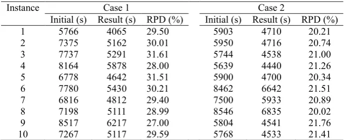
[image:6.595.127.471.317.453.2]The algorithms are coded in C++ and running on a PC (Intel(R) Core(TM) i5-4570, CPU 3.2GHz, RAM 4GB). Table 3 displays the experimental results. The average relative percentage deviation (RPD) is calculated as 𝑅𝑃𝐷: = (𝑖𝑛𝑖𝑡𝑖𝑎𝑙 − 𝑟𝑒𝑠𝑢𝑙𝑡) 𝑖𝑛𝑖𝑡𝑖𝑎𝑙⁄ . For there are more constraints in case 2, the optimizing effect of case 2 is not as good as that of case 1. But the result shows that the proposed TS algorithm can achieve a good performance on both cases.
Table 2. The summary of test cases.
The environment element Case 1 Case 2
Site type 10 10
Site 60 60
Mutex relation between site 55/60 55/60
Fixed resource type 15 15
Fixed resource 160 160
Move resource type 10 10
Move resource 50 50
Job 8 10
[image:6.595.124.472.474.615.2]Activities (in per job) 30 30
Table 3. The performance of the TS algorithm.
Instance Case 1 Case 2
Initial (s) Result (s) RPD (%) Initial (s) Result (s) RPD (%) 1 5766 4065 29.50 5903 4710 20.21 2 7375 5162 30.01 5950 4716 20.74 3 7737 5291 31.61 5744 4538 21.00 4 8164 5878 28.00 5639 4440 21.26 5 6778 4642 31.51 5900 4700 20.34 6 7780 5430 30.21 8462 6642 21.51 7 6816 4812 29.40 7500 5933 20.89 8 7198 5111 28.99 8546 6835 20.02 9 8517 6217 27.00 5804 4541 21.76 10 7267 5117 29.59 5768 4533 21.41
Summary
In this paper, the model RCMPSPTW is established aiming at solving the problem with resource breakdown that may occur during the actual project scheduling. A heuristic algorithm based on SSGS is designed to generate the initial solution and a TS algorithm is proposed to optimize the solution. Experimental results show that the proposed model is feasible and the TS algorithm is effective.
References
[2] A. Lova, P. Tormos, Analysis of scheduling schemes and heuristic rules performance in resource-constrained multiproject scheduling, Annals of Operations Research, 102 (1-4) (2001) 263-286.
[3] O. Lambrechts, E. Demeulemeester, W. Herroelen, Proactive and reactive strategies for resource-constrained project scheduling with uncertain resource availabilities, Journal of Scheduling, 11 (2) (2008) 121-136.
[4] R. K. Chakrabortty, R. A. Sarker, D. L. Essam, Multi-mode resource constrained project scheduling under resource disruptions, Computers & Chemical Engineering, 88 (2016) 13-29.
[5] S. Kreter, J. Rieck, J. Zimmermann, Models and solution procedures for the resource-constrained project scheduling problem with general temporal constraints and calendars, 251 (2) (2016) 387-403.
[6] D. Krüger, A heuristic solution framework for the resource constrained (multi-) project scheduling problem with sequence-dependent transfer times, European Journal of Operation Research, 197 (2) (2009) 492-508.