Tabu Search Solution for Resource Confidence Considered Partner Selection Problem in Cross Enterprise Project

doi:10.4236/jsea.2010.36063 Published Online June 2010 (http://www.SciRP.org/journal/jsea)

Tabu Search Solution for Resource Confidence

Considered Partner Selection Problem in

Cross-Enterprise Project

Hanchuan Xu, Xiaofei Xu, Ting He

School of Computer Science & Technology, Harbin Institute of Technology, Harbin, China. Email: {xhc, xiaofei, xuantinghe}@hit.edu.cn

Received April 1st_{, 2010; revised April 21}st_{, 2010; accepted April 23}rd_{, 2010.}

ABSTRACT

Cross-enterprise project is the main implementation form in multi enterprises collaborative production environment. Minimizing the risk of failure and tardiness caused by the uncertainty of partner’s resources in partner selection is the key problem to ensure success in Cross-enterprise project. In this paper, considering the factors and constraints of sub-project processing times, precedence of sub-project and project due date, especially the resource confidence, a 0-1

integer programming model was presented with the objective to minimize the risk of failure and the tardiness of the project. A project scheduling algorithm was designed to search and evaluate selection solutions, and the project scheduling algorithm was embedded into a Tabu search algorithm to solve the model. Simulation experiments and comparisons with other algorithms showed that the proposed approach was possible to find the optimal solution with a faster speed and higher probability.

Keywords: Cross-Enterprise Project, Partner Selection, Resource Confidence, Tabu Search

1. Introduction

To be competitive in the global manufacturing environ-ment with the rapidly increasing competitiveness, strate-gic collaborations between enterprises are needed in order to meet the market’s requirements for quality, respon-siveness, and customer satisfaction. Dynamic alliance, virtual enterprise, extended enterprise, and supply chain are the major management philosophies for multi enter-prises collaborative production environment. Cross-enterprise project (CEP) management pattern arose as the main implementation form in these management philosophies. CEP is the formation of closer co-ordination in the design, development, costing and the co-ordination of the respective manufacturing schedules of co-operating independent manufacturing enterprises and related sup-pliers [1,2]. There are four stages in CEP life cycle: for-mation, operation, evolution and dissolution. A major issue in the formation phase is to select appropriate part-ners and allocate tasks between partpart-ners. During this process, the core enterprise comprehensively evaluates partners according to cost, quality, credit, delivery time, etc., and then based on certain criteria, find the best combination of partners to collaborate to complete the

project.

Partner selection has attracted much research attention recently, because it is an important function for informa-tion management systems, such as project management (PM), enterprise resource planning (ERP) and supply chain management (SCM). Most of researches about the partner selection problem are based on qualitative analysis methods. However, quantitative analysis methods for partner selection are still insufficient. Many operation research methods, such as analytic hierarchy process (AHP), analytic network process (ANP) and fuzzy syn-thetic evaluation are widely used to the problem, but mathematical models and optimization methods for part-ner selection are still a challenge [3,4]. In partpart-ner selection process, although there are many factors needed to be considered such as friendship, credit, quality, and reli-ability, the cost and completion time are the two key factors and focused on by most researchers.

constraints between enterprises such as contracts, the case that partners can’t provide promised resources on time or in right quality is not able to be completely avoided. When this happens, it will seriously affect the production sche- dule of core enterprise and even cause the whole cross- enterprise project failed. So the confidence level of re-source that can be provided by partners on time and in

right quality which we defined as resource confidence is a

very important factor in the partner selection problem. However, most researchers mainly take into account the cost and completion time, and the objective is to minimize the total cost of the project or the project duration. The factor of resource confidence is neglected in most re-searches.

Yannis and Andreas [5], Sha and Che [6], Mikhailov [7] and other researchers proposed some models and ap-proaches for partner selection by establishing a CEP, where cost, time and distance were considered. However, the other two important factors, the resource confidence and the precedence of sub-project, were not considered in

their papers. As Wang et al. [8] indicates, in the

coopera-tion relacoopera-tionship of sub-projects contracted by partners, it may be represented by an activity network with prece-dence. Thus, the problem could be considered as a partner selection problem embedded with project scheduling.

Naiqi et al. [9] considered the completion time as a

con-straint and modeled the partner selection problem by an integer programming formulation to minimize the manu-facturing cost. The formulation was then transformed into a graph-theoretical formulation and a 2-phase algorithm

was developed to solve the problem. Wang et al. [8] took

into consideration the factors of cost, completion time and precedence of sub-project, described the partner selection problem with a 0-1 integer programming formulation to minimize the total cost of the project. They then devel-oped a fuzzy decision embedded heuristic genetic algo-rithm to find the solution for partner selection. The ex-periments showed that the algorithm was possible to quickly achieve optimal solution for large size problems. Taking into account the same factors and objective as

Wang [8], W. H. IP et al. [10] and Zhibin et al. [11]

sepa-rately proposed branch and bound solutions for partner selection problem in virtual enterprises and their solutions were especially effective to medium or small size prob-lems. In all these papers mentioned above, their objectives were minimizing the total cost of project and didn’t con-sider the impact of resource confidence to project im-plementation risk. To minimize risk in partner selection and ensure the due date of a project in virtual enterprise,

W. H. IP et al. [12] described and modeled a risk-based

partner selection problem. They developed a rule-based genetic algorithm with embedded project scheduling to solve the problem. In their paper, they assumed that each candidate partner had a fail probability of its contracted sub-project. In fact, the fail probability of the sub-project

closely related to whether the partner’s available re-sources were tight or not in the duration of the sub-project. The tighter the resources are, the higher the fail probabil-ity is, and vice versa. However, the production load of partner is varied in different periods, so the available resource and fail probability are also different. They used a whole fail probability for all periods and didn’t consider the difference of fail probability in different periods.

To solve the partner selection problem in CEP, we first describe it with a 0-1 integer programming model con-sidering the factors of process time, precedence of sub- projects, and resource confidence. Then a project sched-uling algorithm is proposed to calculate the project com-pletion time and the time window of each sub-project under a feasible solution. From this, we embed the project scheduling algorithm into a Tabu search algorithm to obtain the optimal partner selection solution. The com-putation results showed that the proposed approach is efficient to achieve the optimal solution.

The paper is structured as follows. In Section 2 the problem and the model are introduced. Then the solution space reduction method and the project scheduling algo-rithm to evaluate selection solution are presented in Sec-tion 3. The Tabu search algorithm embedded the project scheduling is presented in Section 4. Section 5 reports an experimental example and computational results obtained by testing the algorithm on some test instances. Finally, Section 6 presents our overall conclusions.

2. Model for Partner Selection Considering

Resource Confidence

The problem of partner selection for CEP considering resource confidence can be described as follows:

Assuming an enterprise (core enterprise) obtain a big project consisting of several sub-projects. It is not able to complete the big project by itself from its own resources and has to find some partner enterprises to collaboratively finish the project. The partner selection procedure is di-vided into two phases. Firstly, the enterprise determines the payment and some basic requirements for the process time and quality of each sub-project. The partners who can accept the conditions will propose the process time they need to finish the sub-project according to their own capacity. They constitute the candidate partner set. In the second phase, the enterprise comprehensively evaluates all candidates and calculates the confidence of resource provided by the partner for the sub-project. At last the enterprise selects the most appropriate partner for each sub-project. There exists plenty methods to evaluate the individual candidate partner and calculate the resource confidence, for an extensive review we refer to MALONI

and BENTON [3] and BOER et al. [4]. In this paper, we

just focus on the second phase, i.e., how to select partners

according to the resource confidence.

pre-sented by W. H. IP et al. [12] and considering the resource confidence, we present a 0-1 integer programming model MPCPS for the partner selection problem. Suppose that the project consists of sub-projects, there are prece-dence relationship between these sub-projects and they form a precedence activity network

n

H. If sub-project

can only begin after the completion of sub-project , we call project as the immediate predecessor of

sub-project and define the connected sub-project pair

by . For the convenience of description, we

label these sub-projects such th i k . Without the loss

of generality, the final sub-project is labeled as

sub-pro-ct n. Thus, we can define that the completion time of

final sub-pro ct cn is the completion time of the project.

Each sub-project has some candidate partners, for sub- 1, 2,...,n, the are mi candidate partners,

and for the candidate ner

k i i k   i, , i k H

j

project 

at

je

e

re

i

part j of su -project i, its

processing times is qijperiods. The resource confidence

candidate

b

of j to ub-project in period t is d as

( )

ij

d t d tij( ) (0,1] . The due date of the project is

D. To simplify the problem, we assume that the core

en-terprise will select only one candidate to undertake one sub-project.

s i note

and there

The objective is to select the optimal combination of partners for all sub-projects in order to maximize the whole resource confidence of the project and to finish the project within the due date.

The following decision variable is defined.

1 ( )

0 ij x t _{ }



Then the problem can be modeled as follows: MPCPS





           n i m j c t * n q t t τ ij ij ij d x

i n ij

D c β τ d q t x x F max

1 1 1

1 ) ] ] [[ (1 ] ) ( 1 )[ ( ) ( (1) s.t. 1 1

( ) 1; 1, 2,...,

mi cn

ij j t

x t i

   



n  (4) (2)

1 1 1 1

( _ij)mi cn _ij( ) mk cn _kj( ); 1, 2,..., ,_n ,

j t j t

t q x t t x t t c i k H

   



_



_

  

(3)

1 1

( ) ( )

m_n c_n

nj nj n j t

t q x t c

 

 



( ) {0,1} , ,

ij

x t  i j t (5)

where [ ]x _{stands for max{0,w} , [ ]y} _{stands for}

min{1,y} and  is the tard en coefficient.

(1) is the objective function, where

iness p alty

Formula 1

ij

q .

1 t qij _{( )}

ij t d

 

 

ence for candidate 



source confid

is the mathematical expectation of

re-j of sub-project i in

the qij continuous periods, and bbreviated as a Eij

bel-low. onstraint (2) ensures that each sub-project will be contracted to only one partner and constraint (3) is the precedence constraint of sub-projects. Constraint (4) gives the method to calculate the completion time of the project.

It is ob C

vious [ ]y _ar

at

o e

ion

mp

that the operator [ ]x_{and non-}

ot c

PCPS is a c lex

an

3.1

alytical and the objective function is n ontinuous

and differentiable, so it is difficult to treat the model by traditional mathematical programming methods. There-fore, we develop a project scheduling embedded Tabu search (PSTS) algorithm to solve this problem.

3. Solution Space Reduction and Evalu

Algorithm of Solution

Solution Space Reduction

M The partner selection modeled as

combinatorial optimization problem. The number of fea-sible solutions (solution space) is very large, even for a small-scale problem. To simplify the solving process, W.

H. IP et al. [12] defined the concept of inefficient

candi-date and proved that the optimal solution consists without

any inefficient candidate. To efficiently reduce the solu-tion space, all inefficient candidates can be ignored in the solving process without losing the optimal solution. Based on the definition presented by W. H. IP [12] and consid-ering the characteristics of the model MPCPS, we define the inefficient candidate to our model as follows.

Definition 1. For the two candidates j and k o

candidate j is selected to sub-project i at period t

otherwise

f sub- pr

,d

oject i , if _[ min_, max_]

i i

t ES LF

  _[ min_, max_]

i i

t ES LF

  ,

( )

ik ij ik

q q t d t_ij( ) , or q_ik q_ij,d_ik(t)d_ij( )t , then

the candidate j is called inefficient candidate.

It is easy to rove that there exists at least onep optimal

solution which doesn’t include any inefficient candidate. Therefore all the inefficient candidates are not considered in the model without loss of the optimal solution. In

definition 1, min

i

ES is the earliest possible start time and

max

i

LF is the latest allowable finish time of sub-project i.

ngest possible time window _[ min_, max_]

i i

ES LF of

sub-project i is only a part of the whole project time

window [1, ]c , so to judge whether a candidate is

ineffi-cient or no e only need to do the judgment in time

window _[ min_, max_]

i i

ES LF according to definition 1, rather

The lo

n

t, w

-proves th of definition 1 and the effect of

solution space reduction. Let min

i

q and max

i

q be the short-

est and longest process time of sub-project i respectively,

min

1, 2,...,

min{ }

i i i _imi

q  q q q , q max 1,qi2,...,qimi} ,

then min

i

e satisfiability

max _{

i qi

ES and max

i

LF can be calculated with min

i

q and

max _{oject scheduling problem with the}

,

i

q . This is a pr

objective of minimizing project makespan, i.e.

max

PS p an re exists some polynom time

ithms [13]. rec C r Evalua d the m, th ial

tur b ng is selected

algo

3.2 Project-Scheduling-Based Solution n Algorithm

In our TS algorith

tio

e na al num er stri

as code description. Let x[ , ,..., ]x x_{1 2} x_n , where x_iis an

nds candidate

integer between 1 and mi. This sta for that

i

x is selected for sub-project i. Thus, x[ , ,..., ]x x_{1 2} x_n is

called a selection. For exa 3 4] is a partner

selection of a project with 7 sub-projects. In the selection, the candidate 3 is selected for the sub-project 1, and the

didate 4 is selected for the ub-proje

Once a selection fixes the candidates for all sub-pro-jects, to obtain the object function value, a project-sche-

duling-based solution evaluation algorithm PSLP can be

done to calculate the variable values of c and

mp 1 5

c d so on.

le, [3 4

s

2

t 2, an can

n Eij, and

t i i( also the object function value. The procedure of the algo-rithm PSLP is described as follows:

Algorithm PSLP

Step 1: Calculate the earliest starting time ES_i and the

earliest finish time EFi of each sub-projec 

1, 2,..., )n . If do not exist ( ,k i)H, k {1, 2,..., }n

, letion tim e {1, 2,..., k , then ) i

j p e c

F .

i

LS and th

,.. }

n

  , then

}. 0

i

ES  ; Else, ES_i max{EF_k, (k H} .

i i ixi

EF ES q .

: Calculate the p n. Let

,LSn E

late the latest starting tim

St

LF

lat

LF

ep 2

n EF Step 3: C

If do not

ro ect com

n n

c L

H , n , alc n S u

exist ( ,i

e

est finish time LF_i of each sub-project i i( 1, 2 ., )n .

)

k

;

i LFn Else, LFi min{LSk, ( , )i k H LSi

i ixi

LF q .

Step 4: Calculate h sub-

1, 2,.. s l

th ., )n

ot.

e fl me eac

whe i critica

i

oat ti judge

i i

i

FF of ther it project

sub-p (

i i

roject or

and

n FF LS ES .

U ,

cal-If FF_i 0 , then U_c U_c{ }i , Else

{ }

nc

U U  i .

Step 5: For each sub-project in

nc

non-critical

culate the maximu al expectation of

confidence by th step-by-step right-shifted procedure.

nc

m mathematic resource

e

Step 5.1: If U_nc  , then go to Step 6; Else he

non-critical sub-project i from Unc which has the

maximum earliest start time. U_nc U_nc\{ }i ,

Pos

0

get t



,

0 ixi E  .

Step 5.2: For j0 to FF_i 1 Do If _ixi 1

ixi E q  1 ( ) j qixi ix i d ES   i k j

k 



then 1 1 ( ) j qixi

ix ix i

ixi

E d E

q

 







i i

k j

S k ,

Pos j End For.

Step 5.3: Adjust oat time of each immediate pre

ceding non-critical sub-project of sub-project the fl i. Fo-r

, and ( , )k i

nc

k U

  H, let FF_k FF_kPos, go to

St

he maxim thematic ectatio ur

ep 5.1.

Step 6: For each critical sub-project i U c, calculate

t um ma al exp ce

con-fidence,

n of reso 1

0

ix_i ix_i i

k ixi

1

( )

qixi

d ES k



E 

q 





.

Step 7: Calculate the objective function value. F xd( )

m n i  

_



1 1 1

( ) (1 [[ ] ] )

cn

ij ij n

j t i

x t E  c D 

 



  



Step 8: Over.

In the PSLP algorithm, the time window of each sub-

project is calculated first. There,



ES ES_i, _i1,...,LS_i



d



EF EFi, i1,...,LFi



roject set Uc, the

an represent

do

, tha

rge-scale combination optimization problem. rtcomings of the starting time win-

al path, the critical

w and finish time windows of sub-project i,

respec-tively. In addition, the project critic

sub-p non-critical sub-project set Unc

and the float time of each sub-project can also be deter-mined. In the second part, based on the idea of solving the resource levelling project scheduling with fixed project

duration problem and considered the characteristics t

the resource confidence is various in each period and non- critical sub-project has float time, a step-by-step right- shifted procedure is employed to find the time section in which the non-critical sub-project has the greatest mathe- matical expectation of resource confidence. In the pro-cedure, non-critical sub-projects are dealt with in accor-dance with descending order of the earliest start time. At the last part, the objective function value for a selection is obtained.

4. Tabu Search Algorithm Design

The Tabu search (TS) algorithm is an effective method for solving la

one e constringency speed to the fact that, in the widest some common heuristic algorithms which only adapt to special problems and easily sink into local optimal solu-tions. TS has been used on an increasing number of prac-tice problem and has proven to be effective [14,15].

4.1 The Initial Solution

The initial solution is very important to TS and a good is very useful to improve th

timal solution. Considering

feasible time window



ES ES, 1,...,LF



of the sub-pro-

ject, the greater the resource confidence mathematical expectation of the cand date is, the higher the probability

of being selected is, th generation

pro-cedure PINI is designed as the following steps.

Step 1: From sub-project i 1 i

e initial solution

 to n, calculate the

wid-est feasible time window



ES LFi, i



.

Step 2: From sub-project i1 to n, find candidate xi

which has the greatest m

source confidence in all the ca atical expectation of dat of sub-projectes luti

them

andi ire-.

Step 3: output the initial so on x[ , ,..., ]x x_{1 2} x_n . It is obvious that the initial solution is feasible.

4.2 Neighbourhood Structure and Candidate

is s

obt gh changing the value of one bit of the

confidence and the step- by

Solution

Considering the natural number string employed in th

algorithm, neighbor is defined as all feasible solution

ained throu

current solution, i.e., changing a candidate partner of a

sub-project. Moving from the current solution to a solu-tion in the neighborhood is called a move. Therefore, one step in a move can change only one partner of the current solution. Let NB be the neighbor set. Evaluation value of each solution in NB can be calculated by the PSLP algo-rithm. The solution in NB will be selected as the candidate solution with meeting the conditions that it has the great-est evaluation value and the move from the current solu-tion to it is not in the Tabu list.

In the solution evaluation algorithm PSLP described in 3.2, Step 5 is to precisely calculate the maximum mathe-matical expectation of resource

-step right-shifted procedure has high CPU time cost. In fact, if a solution causes the whole project delayed, its evaluation value will be penalized with the penalty factor

 in the Formula 1. Therefore, the solution has very low

probability to be selected as the candidate solution. From this point of view, the following tardiness penalty

aluation procedure of candidate solution CSTPE is

designed.

Procedure CSTPE:

Step 1: Implement the Steps 1-3 in the algorithm PSLP to calculate t

ev

he time window of each sub-project and the e whole project.

he time window

completion time of th

Step 2: If the project isn’t finished within the due date in the solution, then the Step 5 of PSLP will not be run and the subsequent steps will run with t



ES LFi, i



obtained by the Steps 1-3, else the total PSLP

algorithm will be run.

Experiments show that this candidate solution evalua-dure can significantly reduce the time cost and still can find the optim

tion proce

al solution with high probability. Th

sional e number of rows is the length of the t column is the code of the sub-project,

ling,

was found, w

if a solution is

tions (max_tries) and the maximum number of

itera-tio

e detailed analysis is described in the Section 5.

4.3 Tabu List

The Tabu list (TSL) is composed of a two-dimen integer array. Th

Tabu list, the firs

and the second column is the code of the candidate partner corresponding to the sub-project in the first column. The code for every row records a solution in the neighborhood that has been deleted in recent movements. TSL is re-newed according to the criterion of first in, first out.

4.4 Longer-Term Tabu List and Tabu Relaxation

To avoid getting into the local optimum and the cyc two special techniques, longer-term Tabu list (TTL) and Tabu relaxation, are used. TTL is created to dynamically forbid moving overactive nodes in order to get diversifi-cation and help to prevent cycling. The algorithm incor-porates a move frequency table to record the move fre-quency of each sub-project. When a sub-project’s partner is changed, its move frequency is incremented by 1. If a

sub-project’s partner x has been moved more than two

times and TTL is not full, it will be put into TTL. If TTL is

full and if some sub-project’s candidate partner y already

in TTL has a lower move frequency than x, y will be

dropped and x will be added into TTL.

Another technique used is the relaxation of Tabu lists.

If a given number of iterations (relaxed_tries) has elapsed

and TTL is full since the last best solution

hich means the search process has plunged into a local optimal solution or a cycling, both TSL and TTL are emptied and using the current solution as the initial solu-tion to continue the search. Relaxasolu-tion of the Tabu lists will change the neighborhood of the current solution dramatically, which will lead to a rapid downhill move-ment and may lead to new search spaces.

4.5 The Aspiration Criterion and Stopping Rule

The Tabu status of a move can be overruled

feasible and is better than any feasible solution known so far.

In our PSTS algorithm, there are two ways of control-ling the execution time: the maximum total number of itera

ns without improvement of the best known feasible

algo-rithm is stopped when the number of iterations max_tries

and max_unchanged are both attained, or when the

number of iterations doubles max_tries. Therefore, the

total number of iterations is not known in advance, de-pending on the evolution of the search. The combination

of the max_tries and the max_unchanged as stopping

criterion allows the search to continue if the algorithm is exploring a new promising region. Obviously, to give

time for improvement after the restart, the max

_un-changed should be greater than the relaxed_tries.

4.6 Global Description of the Algorithm Algorithm PSTS:

Step 1: Specify the parameters. Set initial

changed, relaxed_tries, set iteration values of , iteration counter for no improve-max_tries, max_un

counter to tries0

ment to unchanged0.

Step 2: Generate an initial solution x using the

algo-rithm PINI and calculate the evaluation value F(x) of

x using the CSE procedu Let the cu nt best solutionre.

*

rre

x x, the best evaluation value _F*_F(x).

Step 3: triestries1, if triesmax_tries and

max_ ,

ged unchanged or if tries  2 

then go to Step 7

unchan

max_tries, , else g

Step 4: If _tries, an ll,

TSL and TTL.

Find the neighborhood NB of

o to Step 4. relaxed

unchanged  d TTL is fu then empty

Step 5: x, calculate the

candidate solution xNB and the evaluatio

solution

n value F x( _NB).

Calculate the best Tabu x_TSL and t

ng piration

he

corre-sponding evaluation value F x( _TSL) from TSL.

Step 6: Consideri the TSL,TLL and the as

criterion, generate the new solution x from xNB and

TSL

x . If _F*_{max{ (F x ), (x )},} *

NB F TSL x x,

*

F

max{ (F xNB), (F xTSL)},

 unchanged 0; else 1

unchangedunchanged  . Go to Step 3.

7: Ou

Step tput _x* _{and is the optimal solutio}

algorithm is over.

If the CSTPE procedure is candidate

so be

le

onsists of 14 sub-projects *

F n,

used to evaluate

lution, then the PSTS will named as PSTS-P. Other-

wise, if just the comp ted PSLP is used, the PSTS will be named as PSTS-NP.

5. Experiments Analysis

The algorithm was coded by JAVA and run on a Pentium Dual 2.2 GHz PC.

The example is a project that c

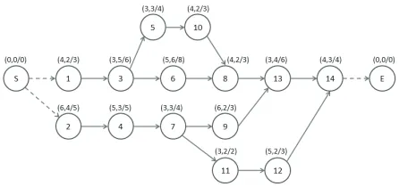
and the core enterprise calls tenderers for the sub-projects. The precedence relationship represented by the active-

[image:6.595.312.535.85.190.2]

on-node network is shown in Figure 1. The numbers

Figure 1. Example of a project represented by active network

in the parentheses are the number of candidates, the shor

he project’s due date is 24 periods and each sub-project t- est process time and the longest process time, respectively. T

has 3 to 6 candidates. The solution space size is 1.05 × 108_.

Through identifying and removing the inefficient candi-dates according to Definition 1, the size is reduced to 2.83

× 107_{. Different candidates may have different process}

time to the sub-project that they bid for. The resource

confidence of the candidate in each period d t_ij( ) is

cal-culated by the fuzzy comprehensive evaluation method,

and where d t_ij( ) (0,1] . For the limitation of the paper

size, the detailed data is omitted.

The setting for the values of parameters is important for

the efficiency rithm. In our algorithm, the “Best_

rate” is used to evaluate and adjust t of TS algo he values of parameters, w

of the PSTS-P, PSTS-NP and B

t it needs much more running time to deal with la

here “Best_rate” is the rate to reach the optimal solution in a certain number of runs. Based on the algorithms of IP WH

et al. [10] and Zhibin et al. [11], considering the character-istics of our problem, a branch- bound algorithm (B & B) is designed to calculate the optimal solution. For different scale problems, the algorithm was run a certain number times according to the scale of the problem with different random seeds for each parameter setting. Therefore, the parameters with the highest “Best_rate” are selected. To the

example in Figure 1, the values of the parameters are

“max_tries = 700”, “max_unchanged = 80”, “relaxed_tries

= 60”, the length of TSL is 18, and the length of TLL is 70.

The result of the example is shown in Table 1, and the

objective value is 0.241.

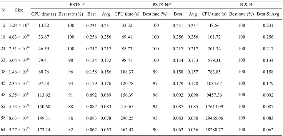
For testing the performance of the PSTS algorithm, we randomly generated some problems with different scales. The comparison results

&B are shown in Table 2. Where “N” is the number of

sub-projects, “size” stands for the size of solution space, “CPU time” is the average computation time of each running.

The B & B algorithm is a kind of exact algorithm and can always find the optimal solution (best rate is always 100%), bu

oce

[image:7.595.54.541.106.248.2]

Sub-project no. Se Resource confidence Table 1. The selected partner list, pr ssing time and resource confidence

lected partner code Processing time Start time Finish time

1 A2 2 0 2 0.82

2 B3 4 0 4 0.80

3 C1 5 3 7 0.76

4 D4 4 6 9 0.55

5 E1 3 9 11 0.60

6 F5 7 8 14 0.72

7 G2 3 11 13 0.58

8 H1 3 15 17 0.63

9 I5 2 15 16 0.69

10 J3 2 12 13 0.72

11 K2 2 14 15 0.83

12 L4 3 17 19 0.82

13 M1 5 18 22 0.91

14 N2 4 23 26 0.87

Table 2. The co arison of PSTS-P, PSTS-NP and B & B

PS B & B

mp

TS-P PSTS-NP N Size

CPU time (s) Best rate (%) Best Avg CPU time (s) Best rate (%) Best Avg CPU time (s) Best rate (%) Best & Avg

12 5.24 × 108 _{13.32 100 0.231 0.231 33.32 100 0.231 0.231 48.56 100 0.231}

18 4.63 × 1010 _{33.67 100 0.256 0.256 69.41 100 0.256 0.256 101.72 100 0.256}

24 7.51 × 1014 _{46.59 100 0.217 0.217 85.73 100 0.217 0.217 201.34 100 0.217}

33 3.04 × 1018 _{79.41 98 0.134 0.132 98.41 100 0.134 0.133 579.31 100 0.134}

38 1.46 × 1021 _{88.76 96 0.158 0.156 108.37 99 0.158 0.157 783.85 100 0.158}

45 2.35 × 1022 _{97.58 94 0.179 0.176 120.78 97 0.179 0.178 1084.67 100 0.179}

48 6.35 × 1024 _{113.62 91 0.092 0.089 156.39 96 0.092 0.090 9457.36 100 0.092}

52 4.53 × 1026 _{130.68 88 0.087 0.083 210.65 94 0.087 0.085 17613.09 100 0.087}

58 8.63 × 1027 _{149.31 86 0.083 0.078 290.25 93 0.083 0.080 29465.06 100 0.083}

64 9.27 × 1035 _{173.24 82 0.062 0.053 362.47 90 0.062 0.056 38280.77 100 0.062}

row fast with the problem size increase. For PSTS-P

complicated and practical problem in

problem of CEP with considering resource confidence,

optimizing ef

g

using the CSTPE procedure to evaluate candidate solu-tions, it can solve large problems faster; on the other hand, PSTS-NP has higher rate to obtain optimal solution. In practice, we can select the appropriate one from the two algorithms according to the different requirements of speed and best rate.

6. Conclusions

Partner selection is a

CEP. Minimizing risk caused by the uncertainty of part-ner’s resources in partner selection and ensuring the due date of the project are important to the success of the CEP. This paper introduces a description of the partner selec-tion problem in CEP. The concept of resource confidence is used to characterize the uncertainty of partner's re-sources, then the non-linear integer programming model (1-5) provides a formal description of the partner selection

where the following features different from conventional methods are considered:

1) The precedence activity network describing the precedence relationship between sub-projects

2) The resource confidence of each partner

A project scheduling embedded TS algorithm for the problem was proposed. Its two variants, PSTS-P and PSTS-NP, focus on computation speed and

ficiency, respectively. The computation results show its potential to solve practical partner selection and project management problems.

[image:7.595.59.540.273.504.2]

REFERENCES

[1] X. F. Xu, “Virtual Organization - the Enterprise Organi- zation Form in the Future,” in Chinese, China Me- chanical Eengineering, Vol. 7, No. 4, 1996, pp. 15-20. [2] H. S. Jagdev a nded Enterprise - A

Context for ction Planning &

n

“A Review of

jidimitriou and A. C. Georgiou, “A Goal

ion in a Global Manu-

ter-Integrated

anu-

plied

n for a Risk-Based Partner Selection Problem

ification, Mo-

206. nd J. Browne, “The Exte

Manufacturing,” Produ

fac

Control, Vol. 9, No. 3, 1998, pp. 216-229.

[3] M. J. Maloni and W. C. Benton, “Supply Chain Partner- ships: Opportunities for Operations Research,” Europea

Man

Journal of Operational Research, Vol. 101, No. 3, 1997, pp. 419-429.

[4] L. D. Boer, E. Labro and P. Morlacchi,

Fact

Methods Supporting Supplier Selection,” European Journal of Purchasing & Supply Management, Vol. 7, No. 2, 2001, pp. 75-89.

[5] A. Yannis, Ha

Programming Model for Partner Selection Decisions in International Joint Ventures,” European Journal of Operational Research, Vol. 138, No. 3, 2002, pp. 649- 662.

[6] D. Y. Sha and Z. H. Che, “Virtual Integration with a Multi-Criteria Partner Selection Model for the Multi- Echelon Manufacturing System,” International Journal of Advanced Manufacturing Technology, Vol. 25, No. 7-8, 2005, pp. 793-802.

[7] L. Mikhailov, “Fuzzy Analytical Approach to Partnership Selection in Formation of Virtual Enterprises,” Omega,

Vol. 30, No. 5, 2002, pp. 393-401.

[8] D. Wang, K. L. Yung and W. H. Ip, “A Heuristic Genetic Algorithm for Subcontractor Select

turing Environment,” IEEE Transactions on SMC Part-C, Vol. 31, No. 2, 2001, pp. 189-198.

[9] N. Q. Wu and P. Su, “Selection of Partners in Virtual Enterprise Paradigm,” Robotics and Compu

ufacturing, Vol. 21, No. 2, 2005, pp. 119-131. [10] W. H. Ip, D. Wang and K. L. Yung, “A Branch and Bound

Algorithm for Sub-Contractor Selection in Agile M uring Environment,” International Journal of Produc- tion Economics, Vol. 87, No. 2, 2004, pp. 195-205. [11] Z. B. Zeng, Y. Li and W. X. Zhu, “Partner Selection with a

Due Date Constraint in Virtual Enterprises,” Ap Mathematics and Computation, Vol. 175, No. 2, 2006, pp. 1353-1365.

[12] W. H. Ip, M. Huang, K. L. Yung, et al. ”Genetic Algo- rithm Solutio

in a Virtual Enterprise,” Computers & Operations Re- search, Vol. 30, No. 2, 2003, pp. 213-231.

[13] P. Brucker, A. Drexl and R. Möhring, “Resource-Cons- trained Project Scheduling: Notation, Class

dels, and Methods,” European Journal of Operational Re- search, Vol. 112, No. 1, 1999, pp. 3-41.

[14] F. Glover, “Tabu Search: Part I,” ORSA Journal on Computing, Vol. 1, No. 3, 1989, pp.