FINITE DIFFERENCE METHOD FOR SOLVING THE SPATIO TEMPORAL DIFFUSION EQUATION IN THE TWO GROUP APPROXIMATION COMPARISON BETWEEN THE SOLUTION BY AN ITERATIVE AND A DIRECT MTHOD EUR 596 e

This document was prepared under the sponsorship European Atomic Energy Community (EURATOM).

EUROPEAN ATOMIC ENERGY COMMUNITY - EURATOM

FINITE DIFFERENCE METHOD FOR SOLVING

THE SPATIO-TEMPORAL DIFFUSION EQUATION

IN THE TWO-GROUP APPROXIMATION

COMPARISON BETWEEN THE SOLUTION BY AN ITERATIVE AND A DIRECT METHOD

by

R.

MONTEROSSO and E. VINCENT!

1964

Joint Nuclear Research Center Ispra Establishment - Italy

I. The finite-dif:ference formulation of the diffusion equations

II. Iterative method (Block Gauss-Seidel)

III. The direct method

IV. Numerical examples

V. Iterative method with variable number of

inner iterations

Appendix A

Appendix B

References

Page

6

9

13

17

23 25 32

Preface

This report describes a part of a numerical program made for the study of the spatio-temporal dynamics of a reactor. The time-dependent two-group diffusion equations are transformed, by the finite difference method, into a system of linear equations.

This program was written for the Reactor TESI which operates in condition of prompt criticality and has :fluxes which increase very rapidly. High accuracy is therefore required in calculating

the fluxes at every time step. For this reason the solution of the system of linear equations was attempted in two ways, by an iterative method, as it is common practice in the nuclear codes, and by a direct method.

This report describes only the two methods used and gives a corn~ parison of their numerical results. A complete description of the program and of the physical problem will be the subject of an-other report.

I. The finite-difference formulation of the diff'usion equations

In this report are described two mathematical methods to be employed in a program for the study of the spatio-temporal reactor dynamics. In this program the time dependent diff'usion equations are solved directly with a numerical method in order to study the variations of the neutronic flux as a function of space and time throughout the core.

This problem is treated in the two-group approximation in order to better evaluate the flux distribution in the reflectors and their influence on the neutron economyo

For simplicity the reactor is imagined as an infinite horizontal slab of finite height H. Along the z-axis the reactor consists of several regions Rk of different physical nature: lower

reflector, non rodded core, rodded core, upper reflector. The two-group diffusion equations of the k-th region~ are the following:

1

aw

- -

_vi<

at ( 1-I)

(2-I)

where:

nk and nk are the fast and thermal diffusion coetti-_{f t}

cients, which are assumed to be constant in each region Rk.

"' = w(z,t) = fast flux

~

=

~(z,r)

=

thermal flux

Bk _{= (1 - ~)•v•Zr(z,t) = prompt neutrons produced} per unity of thermal flwc

ck

₌

_{l•C (z,t)}

₌

_{delayed neutrons produced per cm}3 _{per sec.}

Ek _{= [za(z,t) + zp(z,t) + B}2

•D1]

=

thermal absorption

X-section, rod poison, thermal radial leakage

pk _{= 4t(z,t) = number of neutrons thermalized per unity} fast flux

wk = neutron velocity of the fast group

vk = neutron velocity of the tb.ermal group

The quantities with index k are assumed to be continuous in each region R and may be discontinuous at the interfaces.

k

The fluxes~ and~ and the neutron currents

Dr~

continuous functions everywhere.

• D

£2.

' t

az

are of

The fluxes~ and~ are zero at the lower and upper boundary of the reactor:

~ (o,t) = ~ (H,t) = ~ (o,t) =

t

(H,t) = o

The height of the reactor has been divided into mesh-points

[zlJ

(i = O, 1, 2, ••••• L, L+1) with z

0

=

O; ZL+1

=

H. On each interface between two regions is a point of the lattice, and each region contains at least one point.

'Discretizing also the time-variable t the diffusion equations (1-I) and (2-I) are transformed into:

-m •

W

n - r ·~ n + p ·~n - r ·~

L L -1 t 2 L -1 t 2 L l +1 , 2 t +1

(i = 1, 2, •••••• , L) space index ( n = 0, 1 , 2 , • • • • • ) time index

= \ 2

This transformation is described in Appendix A. This is an implicit scheme. It has been chosen implicit in order to in-sure the numerical stability of the finite difference method without limitation for the time interval 6 t.

(4-I)

The coefficients of the system (3-I); (4-I), which are dependent from the unknown fluxes wand~, have been calculated at the

time level n - 1. The system is in such a manner linearized. The error introduced by such an aJ;?proximation is negligible only for small 6t and for coefficients which vary slowly with the time. The choice of ~t is based on a comJ;?romise between precision and time of calculation.

At every time steI? the coefficients are given new values which are determined according to the temJ;?erature reaction and .the J?OSition of the control rods.

The known terms the fluxes

wn-i

L

distribution of

q and q contain explicitly the values of

L1 l2

and

~?-

1 _{of the J;?receding time step. An initial}

L

fluxes

w

0 _{and ~}0 _{is given at t =}

o.

t t

At every time step the problem is reduced to the solution of the system of 2 x L linear equations in the variables

wt

and ~L.

The solution has been obtained with two me'th,ods, one iterative

II. Iterative method (Block Gauss-Seidel)

The system (I-3);

(I-4)

may be written in matrix notation (see page 25 of Appendix A).

[ Ai+ - St= qi

-M V +A,= q

2 2

The iterative method is as follows:

(II-1)

in the source-terms, of system (II-1) we use the vector~ obtained from the calculation of the preceding time step; the system (II-1) is then solved in

W•

The vector

t

is used in the source-term

Mt

of system (II-2) and a new vector~ is calculated. This is used in the source terms, of (II-1) and so on.

This method is the same as the block Gauss-Seidel iterative method. In fact let us consider the system Ax= q formed by

the two systems (II-1) and (II-2); where

x

=

(1)

and q =~q1) ,

'

~

and the matrix A of the coefficient is partitioned as follows:

A=L-U=

~

ols

~

(II-3)

Applying the block Gauss-Seidel iterative method we have

L. Xr+1 = U • X r + q

A 1j,r+1 = Sq>r + q

1 1

For a time interval sufficiently small (see Appendix A) the matrix of the coefficients A fulfills the -following condi-tions:

att > 0

atJ ~ 0 for i -/ j

N

att

>L

!at

JI

j=1

j,fi

(II-4)

(II-5)

(II-6)

(II-7)

(II-8)

which are sufficient to insure the convergence of the iterative method (see Appendix

B).

The solution of the systems

A r+1

2 cp

must be performed at every iteration; this is obtained by a direct method. The systems ( II-9) and (II-10), with tri-diagonal matrices A1 and A2 , are of the type:

(II-9)

(II-10)

-r X +PX - r • X = U

(1=1, •••

L) (II-11) t t -1 t t · t +1 t +1 L

With

_X

₌

_XL

₌

₀

The known terms UL contain the source-terms.

The solution of system (II-11) is obtained by using the re-cursion formula:

r

t+1

ex ::

t

1\

- r ex

t t-1

ut + rt •

_{'3 t}

_-1.

'3 t

= with ex = B =0

pt

-

r • 0: 0 0

t t-1

This recursive method is suitable for the numerical cal-culation because ext and f3t are of the same magnitude. Only three multiplications, two divisions and three additions are necessary for·the calculation of each spatial point.

In our case the matrix fulfills the conditions:

rt > 0

pt > r _t + r _{L +1}

Therefore we have:

ext < 1

the error ej resulting from the calculation of

xj

is

trans-mitted by the recursive formula (II-12) according to:

e: =ex . e

J-1 J -1 J and for (II-17) we have

e:. < e

J-.1. J

III. The direct method

Rearranging the system

(I-3), (I-4),

intercalating the

equations of

(I-3)

with the corresponding equations of

(I-4),

we obtain a system with a pentadiagonal matrix of the coefficients. This matrix can be partitioned into (2 x 2) submatrices according

to the following scheme:

-

-p -s -r 0 11 1 21

-m p 0 -r

1 12 22

-r 0 p -s -r 0

21 21 2 31

0 -r -m p 0 -r 12 2 22 3~

~~~

-rL,1 0 0 -r _L,2

--

-The generic equation of the system is:

-R • X + P • X -R • X

L t -1 L L L +1 L +1

where

. X.

L

=

p -R

1 2

R P -R

2 2 3

(1 = 1, ••• ,L)

and where RL and PL are non singular 2 x 2 matrices.

( III-1)

=A

The direct method of solution employed for the equations (II-11), with the recursion formula (II-12), may be generalized for

this case of equation (III-3). In fact the matrix A, if con-sidered as consisting of 2 x 2 submatrices, is tridiagonal.

The recursion formulae are now

X = A • X + b

t t t +1 L

where the matrix A is

L

A =

(pt

- R • A

)-1 •

R

t l t-1 l +1

and the vector b is

L

b =

(pt

- R • A

)-1 • (q

+ R • b )

t t t-1 l t t-1

The boundary conditions are:

and therefore we have A

= O and b

= O

0 0

Starting from A and b we can calculate forwards all the

0 0

(III-3)

(III-4)

(III-5)

At and bt, and with these, starting from XL+₁ , we can calculate

backwards all the

x

L

For this method it is necessary to perform the inversion of the L matrices (P - R • A ).

NOTE:

In order to avoid the cumbersome operation of inverting these L (2 x 2) matrices we tried the H-met.hod of Schechter, where it

is sufficient to invert only one matrix. The matrices R are L diagonal and therefore directly invertible. We multiply the system (III-2) by R

R =

I

'

'

The matrix of the coefficients then becomes:

P' R'

1 2

I P' R'

2 2

I P' R'

3 3

with P' = R-1• P •

t t L ' R' =

-R-1

• R •

t +1 t t +1'

The recursion formulae of the H-method are:

'X. = q_' - P 'X - R' • XL +

1

t -1 l. 1 1 t +1

where H = H • pt - H • Rt

t t-1 L t-2 t

w

= H • q -

w

t t-1 t t-1

and for the boundary conditions

H = I

0

H = pt

1. 1.

(See Schechter: "Quasi-Tridiagonal Matrices and Type-insensitive Difference Equations")

With this method, however, we obtain unsatisfactory results because of the propagation of the rounding errors:

e = -Pt • e - Rt • e:

IV. Numerical examples

The two methods above described are part of a numerical code to be employed on the IBM 7090, and which is rrade for the study of the spatio-temporal dynamics of the Reactor TESI.

This reactor operates in the following way: from being critical at a very low power it is made prompt critical. The flux rises very rapidly, and, as the reactor is not cooled during the

transient, the temperature in the core rises accordingly. The core has a large negative temperature coefficient, therefore when a certain value of the flux is reached the reactor be-comes undercritical and the flux decreases very rapidly.

For testing the two methods of calculation we introduce step-wise a reactivity p = 0,1

%.

The control rods in this parti-cular case are supposed to be extracted instantaneously and Zp (rod equivalent poison, see page 3) is reduced instantaneous-ly and uniforminstantaneous-ly all over the core. This causes a transient of

10 the order of 0,5 sec, during which the flux changea from 10 to

18 n

10 cm2sec• For a given time interval 6t, chosen for the numerical calculation, the increment of the flux in 6t is very large.

With the iterative method the thermal flux at the time tn is taken as a first estimate for calculating the :n.uxes at the time tn+1 = tn + 6t. Therefore the choice of 6t influences

very much the effectiveness of this method: the greater 6t, the greater is the number of inner iterations necessary to reach the wanted precisiono

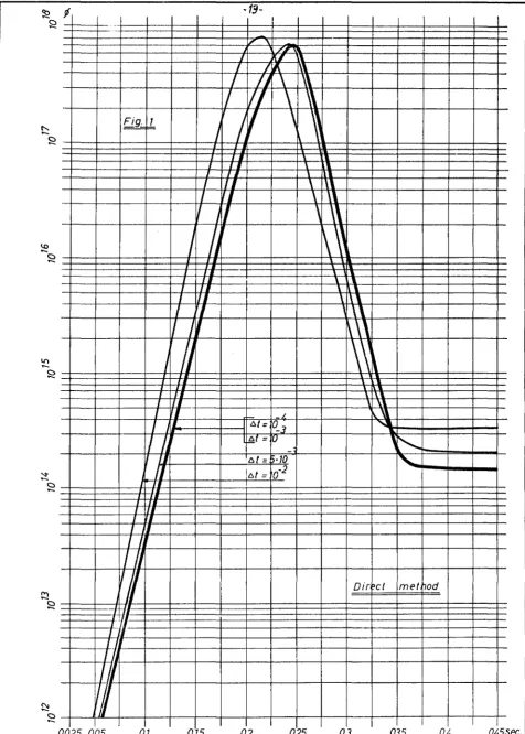
Many tests were made using several 6t in the range:

With the direct method and with various ~t contained within these limits the fluxes and teIIl]?eratures have no appreciable variation. In Fig. 1 are the curves of i(t), (i is the

thermal flux averaged throughout the core). These curves were obtained by both the direct and the iterative method, the

'

iterative method with enough iterations to obtain practically the same results as with the direct method. For ~t less

than 10-3 sec the curve has no appreciable variation, for ~t > 10-3 sec the curve tends to be deformed. This is due to

the fact that the variation of the temperature-dependent physical parameters during the interval ~t is no longer negligible.

In Fig. 2 are plotted the curves ~(t) for ~t = 10-3 sec, calculated with the direct method and with the iterative method with 2,

3,

4,

5,

and

6

iterations. Table 1 contains

the numerical values of some points of these curves.

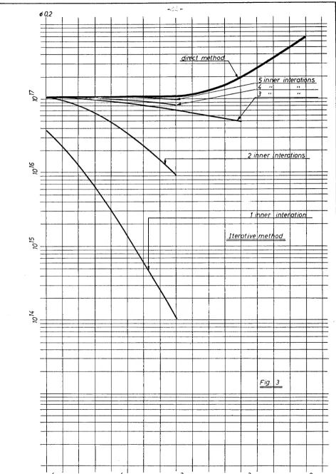
Fig. 3 contains the values of the flux calculated at a transient time value of 0,2 sec. These are plotted against the time

interval ~t. The curve of the direct.nethod remains at a con-stant value for all ~t < 10-3 sec. The other curves, corres-ponding to the iterative method, tend to the same value for decreasing ~t. The greater is the number of inner iterations, the greater is the ~t for which the wanted precision is

I i i ,I

I Ill.. \1

I

"

\

1

!/

_//

_\

Fig . 1

/

I

'

1 =

=

) ~

' ''.

.

I _{I •} \

I _{I •} \

I I • \

I II \

I

I

\

I

_J/

'

\

)

h

\~

'

'.

\ \

'

'.

'

-I I • \

•

I

,.

\

•

I

,.

\

'

II \ \\

I/ _{1 \ \}

If

\\\

J

_.

J

_-

\

\\

'

.

• _'

'

,.

'

I

•

\ \

I f I 1 I

I I _ / \. l

I

j _{I Al=}

G_3

'-'

_•

I

'

l~t = '0

,,

-6( = HO

'--6! = o-2

I ' ' I I I I

I

I

I/

_{Dir he/ met nod}

' I I I I I

I

I' A I

[image:21.569.50.527.88.755.2]

I / ' 1 .I' \

J

I

V\

\

v-"

//

/\

\

\

I/

Fig:_2._

I/

I

'

\

'

I

, ,

' · -

-,

" '

I I I _{' I} I I

• I I

'

I

I

'

V

I _' \ \ /\

II I

\ \

_{I '}

II I

\

\/

\

//

I

'~\

'

_·-,__

• 'tl I

---• ,

.

' _'

----.-•

I I 'tl I \

I I I I \

' j I I \ \ ~

I I I I

'

_\ \

II I

\ \

'

I/

I

I

'

\

\

drect methpd j

I

_I

I

,,

\

I

I

j

_\

" , 11 I

'

•1 I I I! I I

II -, I I • _'

I I I I I

'

II I I \

'

II I I \ I\ \

II

I

_\

_\ 1

'/

'

I

\.\

I\.

l '/

I

"--~ _I'.. ...

__

• I ,

.! I I

Ill I F

I I I I

-

-

II I

" j

I

'I I

I

I

I

Inte ativi me, hod

I

I 7 !/'Jn, r 1n erati f).fl__

I ~ " tn terat, vns

I 11 " _{· - --}~

,

I I

I I I

I I

I

I

-

---I

I

I

Time inter vat l (::,. 7 ~-3 ser.

j

j

--

r

l NU~AER OF INNER ITERATIONS ~EThOO

! _{TIME 2 3} ---·-_{4 5}

_t

₆

---i

o.

O.lOOOOE 11 ~.DJOOE 11 O.lGDClOE 11 0.10000E 11

I

O.lOOOOE 11

o.1aoooe

11

o.osoo

0.32645E 12 0.49922E 12 J.57849E 12 0.60797E 12 0.61816E 12 0.62332E 12

0. 1000 C. 10069E 14 Q.23574E 14 0.31651E 14 0.34959E 14

I

o.36141E 14 0.36746E 14

0. 1500 0.31109E 15 0.11099E 16 0.17254E 16 0.20022E 16 0.21043E 16 0.21572E 16

0.2000 Q.94310E 16 1.4S360E 17 C. 82754E 17 Q.98611E 17 0.10448E 18 C.10753E 18

0.2500 0.19746E 18 C.56132E 18 0.64856E 18 0.66439E 18 0.66783E 18 0.66956E 18

0. 3000 0.54986E 16 0.58789E 17 0. 20634E 17 0.14619E 17

I

0.13063E 17 0.12359E 17

0. 3500 0.14069E 17 :).54414E 15 0.27716E 15 0.23967E 15 I 0.23035E 15 0.22640E 15

0.4000 O. 30090E 15 0.15843E 15

I

0.15747E 15 0.1576/JE 15 0.15774E 15 0.15779E 15

0.4500 O. 15539E 15 Q.15541E 15 0.15626E 15 0.15663E 15 0.15684E 15 0.15690E \5

RESULTS OBTAINED WITH DELTA T = 0.001

TAB• 1

N

~

--~

dire et m thoc ~~

\

/

"

~

5 inr: Pr in erotic ns_

~ ...-- 4

..

..

i - - - 3

..

..

--

, --. / ~ ...

-

-

_/ ...

---

-

_'

"

~

""'"'

"

~

_"

"

'\

_"

2 i ~ner ·nterc tions

~

I\. ' ' _' .'\. \. .. \

I\

1 I nner inte, at ion

\

_{Jte, ptive metl od}

f\

'\

' '\

I\

"

_\

'

\.

\

Fig. 3

[image:24.570.54.526.82.747.2]

v.

Iterative method with variable number of inner iterations

The number of inner iterations necessary to obtain a given pre-cision is proportional to the difference

t:. ~ =

'i (

tn + t:. t ) -

i (

tn )

Butt:.~ varies with tn during the transient. Therefore the program was made to iterate until

-n - ~

~L t-1

~ L

< e;

where i is the index of the inner iteration and e: is the greatest admissible relative error. The maximum number of allowable iterations is fixed, and when this maximum number is reached the program stops iterating even if the wanted precision is not yet attained. By this method it is possible

to avoid a number of useless iterations in some parts of the transient, and, by increasing the max. number of allowable iterations, to reach any wanted precision.

TABLE No, 2

,:\ t max. e; time time

number of _{direct iterative}

iterations

2• 1

o-

3 ₆ 10-4 _{1,066 23} II ₃₈

"

2•1

o-

3 8 10-4 0,213 23 tl

44

II

10-3 ₆ 10-4 _{0,0283 41} II _{1 03}

'

"

5.1

o-

4 ₄ 10-4 _{0,024 1} t ₁₅

"

1 32

"

10-4 ₃ 10-4 _{0,00306 5 48}

'

"

₅

'

₄₄

"

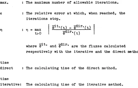
[image:25.571.49.538.535.726.2]

TABLE No. 2 contains for various ~t:

max. : The maximum number of allowable iterations.

time direct

time

: The relative error at which, when reached, the iterations stop.

: ~ = max t>O

iit•(t) _ ~ir.(t) ~ir.(t)

where ~it. and ~ir. are the fluxes calculated

respectively with the iterative and the direct methodo

: The calculating time of the direct method.

[image:26.571.63.517.154.445.2]

Appendix A

The diffusion equations of the Rk region are:

1

aw

-vt-

at (a-1)

(a-2)

The space is divided into mesh-points [zt

J

(i=O, 1, 2, ••• L, L+1).

On each interface between two regions is a point of the lattice, and each region contains at least one point.

The mesh increment is 6t = zt+₁- z~ For all the points 1=1, 2, ••• L

the equations (a-1) and (a-2) must be integrated in the inter-vals

z

1 ~ z ~ zt and z ~ z ~

z

+ 1

t-2 t t 2

i-1 1+1

• ,

1-!

i+!

For the sake of brevity only the integration of equation (a-1) is reported here:

z

t

/

1

aw

- - •dz

w at

Z 1

t - 2

-

[

D -

ch!r]

- f az z _

t

_ [.nf

aw]

az

Z 1 t - 2

z

t

-J

(A• \If - B•cp - C) dz

z 1

t - 2

zt+i

~

at •

dz =

[n aw

J -

[n at

J - /

(A •

t -

B • cp -

c)

dz

w

at

f

az

f

az

\+!

\+

zt

z

t

where

are respectively the left and right limit of f(z) in z = z .

t

(a-4)

Adding (a-3) and (a-4) and remembering that fluxes and currents are continuous we have:

ow

The derivatives

oz

are calculated with central differences; the integrals are approximated according to the formula:

z + 1.

t 2 _6.

6.l

I

f(z) dz = f-. - + t-1

f:"•

t

2 L 2

z

_i-t

The derivatives with respect to the time are approximated according to:

(a-5)

(a-6)

Equation (a-5) then becomes:

6t 1. [

J

6t

• -=-

+ A • ljfn - B • cpn - C •

-2 z 2

If zt is a point internal to ~ then D"" 1. = Df 1. = D';. •

J. t -2 t +2 J.

The functions A, B, Care continuous in zt and equation (a-8) therefore becomes:

6 +6 ,,,n-1. 6 6.

t -1 L

J

<pn =

[ck

+ 'f L

J (

l

-1. + 1. )

2 t t wk. 6.t 2

l

If zt is a point on the interface between Rk-1.and ~ it is

same for B, C, w.

t+

(a-8)

Equation (a-8) therefore becomes:

+ (

--1-

+

A~)

£\i.]

ljr~-~ -f:it L 2 L

(a-10)

Integrating equation (a-2) with the same proceedings we obtain the two following expressions:

for z internal to

R:

t k

Dk

_t_ • q,~

6 1,.-1

t-1

[

6

t-1 + 6

t]

cpn - F.L.... • "1nt =

t +1 2

(a-11)

for zt on the interface between Rk_

nk-1

- _.L._ 0 qi"

t-1

I::.

t-1

+ (

1

+Ek).~]·

qi"

Vk•l\t l 2 t

=

t

n-1

<pt 6_{t -1}

. - +

2

1

Ek-1) At-1

----+

• - +

k-1 • l::.t L

2

vt

AL)

• -₂ • "'" = _t.

.

-

(a-12)

2

The finite-dirference equations obtained by this method are of the type:

- r

t

+ p t - t t - s <p

t1 t-1 t1 t Lt t+1 t L

(a-13)

- m

t -

r m + p q> - t q>

t t t2yt-1 t2 t L2 L+1

(a-14)

(i = 1, ••• ,L)

where

r

=

t

=

r

=

t

=

0

:1.1 L,:1. :1.2 L,2

and t = r

The matrix of the coefficients of the system (a-13) and (a-14) is then:

p -r -s

11 21 1

-r p -r -s

21 21 31 2

~~~

~

-r _L-1,1. p _L-1,1 -r _{L,1 -s}

L-1

[:f.}

-rL 1 _PL1. -s

L

'

)

A =

-M A2 -m ₁ p12 -r ₂₂

"'."ID -r p -r

2 22 22 32

~~

-mL-1 -rL-1,2 PL-1,2

-mL -r _L,2

where the entries on the main diagonal are all positive; and all the other entries are~

o.

The tridiagonal matrices A1 and A2 are definite positive as they

are symmetrical and as their diagonals are dominant and with positive entries.

The diagonal matrices Sand Mare non-negative.

-r 1,fl p

In order that the entries of the main diagonal of the total matrix A are strictly dominant it is sufficient that

1

- - - + Ak > Bk

J: •

tit l L

L

This condition is normally satisfied.

(a-15)

Appendix B

Here below are some definitions and theoremsnecessary to demonstrate that the iterative method (Block-Gauss-Seidel) converges.

Def. 1: It is called "Spectral Radius" p(A), the greatest modulus of the proper values of the matrix A:

p(A) = max

jAt

I

i = 1, N

Def, 2: A matrix A is:

2.a Convergent if the sequence of matrices A, A2

, A3 , • • •

converges to the null matrix

o.

2.b Non negative

real and a .. ~ Ov

l. J

A~ O if all the entries are

2.c Strictly diagonally dominant if t'or all 1 = 1, •••• ,N it is

N

lat

tl

>

L

lat

j

I '

(2.c-1)

i=1

i/j

from (2.c-1) follows evidently

N

\ latj I

< 1 •

Def.

3:

The splitting of a matrix A

A= E - F

is a regular splitting if Eis a non-singular matrix with E --1. ~ 0 and if F ~ O.

Theorem 1 - The necessary and sufficient condition for A to be convergent is:

p (A) < 1

Theorem 2 - The spectral radius p (A) of an arbitrary matrix A fulfills the relation

N

p (A)

~

max. \ latJI i=1 ,N /__,

j=1

Coroll~trY - Let A be a strictly diagonally dominant matrix; 1

let D be a diagonal matrix D =(aLL), then the matrix

B = I-DA is convergent.

In fact the following relation is fulfilled:

p (B) ~

N

max. \ i=1,N L

j=1 j;6i

I :~~I

< 1

Theorem~ - If A= E - Fis a regular splitting of the matrix A and A-1 _{~ 0 then}

- - - < 1

1 + p (A-1_F)

Therefore the matrix E-1

• Fis convergent and the

iterative method

converges ror any initial vector

x

0 •

This last theorem is interesting for our case. In fact the matrix A of the system in study fulfills the following conditions:

N

att >

\

)

lat

JI

L.i

( see II. page 6) j=1

j;ii

therefore, for theorem 3, A-1 _~

_o.

The splitting A= L - U is regular, because the following conditions are fulfilled:

u ~ 0

t

J

i.e.

u

~ 0

1

_{t t}

> 0 1 ~ 0 j;ti (see II. page 5)

tJ

N

1

>L

I\JI

t

t

and, again for theorem 3, they give L-1 _~

_o.

Therefore, for theorem

4

the iterative method of II. is

convergent.

(The theorems 1, 2,

3,

4

are respectively the theorems

AIREK:

COHEN, E.R.:

FOX, L:

KAPLAN, S • :

P.D.Q.:

RIGHTMYER, R.D.:

SCHECHTER, S.:

STAB:

VARGA , R.S.:

WACHSPRESS, E.L.:

WANDA:

References

"Generalized Reactor Kinetics Code"; Atomics International, No. 4980.

"Some Topics in Reactor Kinetics";

Geneva Conference 1958, Volume 11, P/629 USA.

"Numerical Solution of Ordinary and Partial Differential Equations";

Pergamon Press·- 1962.

"Some New Methods of Flux Synthesis"; N.S.&E. 13 - 1962.

"An IBM-704 Code to solve the Two-dimensional Few-Group Neutron Diffusion Equations";

WAPD-TM-70.

"Difference Methods for Initial-Value Problems";

Interscience Publishers, Inc., New York.

"Quasi-Tridiagonal Matrices and Type-insensitive Difference Equations; AEC Computing and Applied Mathematics Center - TID-4500, NY0-2542.

"A Kinetic, Three-Dimensional, One-Group Digital Computer Programu;

AEEW-R.77.

"Matrix Iterative Analysis"; Prentice-Hall, Inc.

''Digital Computation of Space-Time Variation of Neutron Fluxes";

KAPL - 2090.