Munich Personal RePEc Archive
European Banking Integration under a
Quadratic Loss Function
Mamatzakis, E and Koutsomanoli, A
University of Piraeus
September 2009
Online at
https://mpra.ub.uni-muenchen.de/19379/
European Banking Integration under a Quadratic Loss
Function
Anastasia Koutsomanoli-Filippaki*
Emmanuel Mamatzakis**a
December 2009
Abstract
European banking markets have become increasingly integrated in recent years, but barriers to full integration, especially in retail banking, still remain. This paper covers a gap in the literature by providing a first insight into the process of financial integration in the European Union (EU) in terms of convergence in the speed of adjustment of cost inefficiency to equilibrium level. We employ a quadratic loss function specification based on forward-looking rational expectations to model the underlying dynamics of efficiency scores in the banking industry of the EU-15 region over the period 1998-2005. Results show that there is considerable variation in the speed of adjustment across banking systems, while over time it also appears that continuing efforts to advance financial integration have not as yet led to an improvement in the speed of adjustment to the long run equilibrium.
JEL Classification: D24; G21; L25
Keywords: Speed of adjustment, rational expectations, cost inefficiency.
a
Corresponding author:, ** * Department of Economics, University of Piraeus, Karaoli & Dimitriou St. 80, 185 34 Piraeus, Greece. e-mail: [email protected].
1. Introduction
In recent years the European Union (EU) has been transforming rapidly into a
more competitive and integrated economic region. Initiatives, such as the
harmonization of banking and other financial services legislation as part of the EU’s
Single Market, the establishment of the European Economic and Monetary Union
(EMU), and the ongoing implementation of the Financial Services Action Plan
(FSAP) have helped reducing the barriers to cross-border trade in banking services,
thus, enhancing the degree of financial integration. EU deregulation has also
facilitated the environment in which technology and other bank strategic drivers have
become operationally more important (European Commission 2001).
Indeed, substantial progress has been achieved over the years, though this
progress has not been uniform across different segments of the market. Despite a
sustained legislative drive at EU level that led to substantial integration and
harmonization of money, bond and equity markets (Emiris 2002; Hartmann et al.
2003; Baele et al. 2004; Manna 2004; Guiso et al. 2004; Cappiello et al. 2006),
banking integration still faces significant barriers. These barriers arise from national
economic conditions, culture, language and differences in fiscal and legal systems
(ECB 2000; Berger et al. 2001; Buch and Heinrich 2002; Berger et al. 2003). In
particular, the integration process has clearly been slower in the retail banking area
due to the traditionally strong local nature of these activities (Cabral et al. 2002;
Heinemann and Jopp 2002; Eppendorfer et al. 2002; Schuler and Heinemann 2002).
The establishment of the Monetary Union has led to some convergence in the levels
still exist, suggesting that market segmentation remains strong thus impending
banking integration (Cabral et al. 2002; Sørensen and Gutiérrez 2006).
European banking integration is of particular importance as it could positively
contribute to economic growth by removing frictions and barriers to exchange, and by
allocating capital more efficiently (Baele et al. 2004), while, on the other hand, it
could mitigate negative effects derived from systemic risk (Goddard et al. 2007).
After all given that banks are major players in the euro area financial system
achieving homogeneity with an integrated banking sector would improve the
effectiveness of the monetary policy transmission mechanism in the euro area (Cabral
et al. 2002).
European integration has also implications for: the competition in banking
markets, the nature of long-term borrower-lender relationships, and the links between
ownership structure, technological change and bank efficiency (Goddard et al. 2007).
In addition, Molyneux et al. (1997) argue that the formation of a single financial
market place would improve bank’s efficiency.
The topic of European financial integration is not new as it remains at the
forefront of economic research for some years. A plethora of studies in European
financial integration have employed different approaches, using various types of
convergence and dispersion measures (see Cabral et al. 2002; Sørensen and Gutiérrez
2006; Casu and Girardone 2004; 2006). Several studies have examined the degree of
homogeneity across EU banking systems in terms of cost and profit efficiency, with a
Altunbas et al. 2001; Lozano-Vivas et al. 2001; 2002; Biker 2002; De Guevara and
Maudos 2002; Maudos et al. 2002; Vander Vennet 2002; Casu and Molyneux 2003).
In this study, we depart from the traditional efficiency literature, and apply a
multi-period forward looking rational expectations specification to measure the speed
of adjustment to the optimal cost level in fifteen EU countries, namely Austria,
Belgium, Denmark, Finland, France, Germany, Greece, Ireland, Italy, Luxembourg,
Netherlands, Portugal, Spain, Sweden and the UK, over the period 1998-2005.
Moreover, we focus on the degree of homogeneity, and hence implicitly on the degree
of integration, as measured by the speed of adjustment to equilibrium and its
evolution over time in the period 1998-2005. In detail, we opt for the stochastic
frontier analysis within a translog cost function framework, so as to derive
bank-specific inefficiency scores, while as a second step we apply a multi-period forward
looking rational expectations specification to measure the speed of adjustment to the
optimal cost level. In particular, using a dynamic panel model we opt for a quadratic
loss function to account for adjustment costs between the current level of inefficiency
and the optimal one. To this end, the adjustment of banks’ costs is seen as a dynamic
process based on rational expectations, and not as a static procedure. This idea first
came up in the literature of aggregate demand (Cuthbertson and Taylor 1990; Mizen
1994), while Huang and Chen (2006) follow a similar methodology in banking.
The banking sector is usually found to be the least integrated segment of the
European financial system and therefore we should a priori not expect to find a
common speed of adjustment across countries (Sørensen and Gutiérrez 2006).
inherently heterogeneous due to historical differences in market structures, bank
supervision and regulation, and legal traditions, while anecdotal evidence suggests
there are considerable difficulties in reducing heterogeneity or integrating markets via
financial deregulation. This is confirmed by our findings that show different paces of
banking adjustment across countries, providing insights of a lagging integration
within EU banking. Moreover, over time results show that the launch of the euro in
2002, along with the intensifying efforts to achieve a higher degree of financial
integrations, have not had a crucial impact on the speed of adjustment of banks.
The rest of the paper is organized as follows. Section 2 analyses the theoretical
specification, while Section 3 describes the data used in the analysis. Our main
findings are presented in Section 4, while some conclusions are offered in the final
section.
2. A theoretical specification - the efficiency scores
under a quadratic loss function
Firstly, we employ the stochastic frontier approach (SFA), as developed by
Aigner et al. (1977) and Meeusen and Van den Broeck (1977), to estimate cost
inefficiency. According to the SFA, total cost follows the following specification:
TCit = f (Pit, Yit, it, Zit) + vit + uit (1)
where TCit denotes observed total cost for bank i at year t, P is a vector of input
prices, Y is a vector of outputs of the firm, is a vector of fixed netputs and Z stands
components. The first one, vi, corresponds to the random fluctuations and is assumed
to follow a symmetric normal distribution around the frontier, while the second one,
ui, accounts for the firm’s inefficiency and is assumed to follow a half-normal
distribution.
For our cost efficiency function, we opt for a translog specification. This
representation gives:1
lnTCi = 0 + i
i i P a ln +
i
i Y
ln
i + ½
i j
i
ij P Pj
a ln ln + ½
i j
j
ij ln iln +
i j
j i
ijlnPln +
i
i iln +½
i
ijln ln
j j i N N + i j j i N P ln ln ij i j j i N Y ln ln ij + i i Z ln
i +kDi 1t ½
2 2t +
i i
i
i t Y
P
tln i ln
i +
i
i
N tln
i + vi + ui (2)
Standard linear homogeneity and symmetry restrictions in all quadratic terms
are imposed in accordance with economic theory, thus ij= ji; ij= ji; ij= ji,
ij= ji, i, j, while we also include both country and time effects. The cost frontier
can be approximated by maximum likelihood, and efficiency levels are estimated
using the regression errors. Jondrow et al. (1982) show that the variability, , can be
used to measure a firm’s mean efficiency, where 2 = u2+ v2.
Firm level inefficiency for the exponential model is then derived from the
following function2:
1
For simplification, we omit the subscripts for time (t).
2
The normal-exponential model comes from: f(u) e u, where E[u] 1and
2
2 1
] [u
) / ( ) / ( ] / [ v v v i i z z z u
E (3)
where z = - , is the standard normal cumulative distribution function and (.) is
the density of the standard normal distribution.
As a next step, the dynamics of inefficiency scores derived from the first stage
are modelled using a forward-looking rational expectations specification similar to the
one found in the optimal money demand literature (see Cuthbertson and Taylor 1990;
Mizen 1994; Huang and Shen 2002). According to this approach the typical bank is
assumed to minimize the conditional expectation of a discounted quadratic loss
function (L). This objective function takes the form:
2 1 2 2 * 1 1 ) ( )
( t i t i t i t i
n
i i
t D InC InC InC InC
E
L , (4)
where Et is the conditional expectations operator on the information set at time t, D
denotes a discount factor less than unity, and i ( i=1, 2) are the non-negative
adjustment cost coefficients. More specifically, 1 represents the disequilibrium
parameter, measuring the deviation of actual costs InCt+i at time t+i from its optimal
(long-run equilibrium) value InCt*i, while 2 counts for the short-run adjustment
(transaction) between any two consecutive periods.
Taking a partial derivative of equation (4) with respect to InCt+i and
rearranging gives the following equation for operational costs:
n i i t t j t
t InC D D E InC
InC (1 )(1 ) ( ) ( * )
where is the stable root of the Euler equation and its value lies between zero and
one.
We assume that InCt* approximates the functional form of the desired
minimum inefficiency. Here, we assume that this functional form follows a simple
stochastic process:
t t
t InC
InC* *1 , (6)
where t is white noise.
The reduced form cost equation on the basis of (5) and (6) can then be
expressed as:
t t t
t InC InC
InC * 1 , (7)
where *
t
InC is function of D, , and the parameter of equation (6).
The above equation shows the identification of the underlying dynamic effect
as measured by . In detail, captures the persistence of inefficiency scores over
time, whilst 1- reflects the adjustment speed to equilibrium. The values of range
between zero and unity. The higher the value of the longer the suboptimal
inefficiency level persists, resulting in slower adjustment to the optimal cost level. A
firm having a zero value of means that it could correct its past-period inefficiency
instantly, while a unit value of corresponds to a bank that never adjusts its
3.
Data description
Our data includes commercial banks operating in EU-15 countries that are
listed in the IBCA-Bankscope database over the period 1998 to 2005. After confining
our analysis to credit institutions that report positive equity capital and reviewing the
data for reporting errors and other inconsistencies, we obtain an unbalanced panel of
5,568 observations, which includes a total of 883 different banks. As a result, our
sample is quite extensive and covers the largest credit institutions in each country, as
defined by their balance sheet aggregates.3
While there continues to be a debate about the definition of bank inputs and
outputs, we follow along the lines of the traditional intermediation approach as
suggested by Sealey and Lindley (1977), which views banks as institutions that
collect deposits, using labour and physical capital, to transform them into loans and
other earning assets.4 In particular, regarding input prices, the price of labour is
proxied by the ratio of personnel expenses to total assets, while the price of deposits is
defined as the ratio of interest expenses to total funds. The output vector includes
loans (defined as total loans net of provisions) and other earning assets, while total
cost is defined as the sum of overheads (personnel and administrative expenses),
interest, fee, and commission expenses.
3
The year and number of included banks are: 1998:586, 1999:633, 2000:673, 2001:714, 2002:769, 2003:807, 2004:710, and 2005:676. The additions to the sample are not necessarily new market entrants, but rather successful banks that are added to the database over time. Exits from the sample are due primarily to lack of updated data, mergers with other banks or bank failures.
4
We also specify physical capital and equity as fixed netputs. The treatment of
physical capital as a fixed input is relatively standard in efficiency estimation (Berger
and Mester 1997), while the level of equity is included so as to account for different
risk preferences of banks and to control for bank’s insolvency risk (Mester 1996;
Berger and Mester 1997). If financial capital is ignored, the efficiency of banks that
may be more risk averse than others and may hold a higher level of financial capital
would be mismeasured, even though they are behaving optimally given their risk
preferences.5 Apart from this, a bank’s capital directly affects costs by providing an
alternative to deposits as a funding source for loans (see Berger and Mester 1997).
Moreover, to allow for the effect of country features on bank’s underlying
technology, we also include country-level variables in the estimation of the stochastic
frontier, which may be associated with the variations of inefficiency measures across
banks and may affect incentives and managerial decisions. In other words, by
introducing country-specific variables in the estimated cost frontier, we are able to
attribute differences in banking sectors across countries to the characteristics of the
operating environment that are beyond the control of bank managers, thus effectively
conditioning the frontier of the banking sector in each country in a way that is
amenable for cross-country comparisons of bank performance.
These variables include: the Herfindahl index, capturing asset market
concentration, the average capitalization ratio to proxy for regulatory conditions, the
logarithm of bank assets to control for bank size, the intermediation ratio that is
defined as the ratio of total loans to total deposits to capture differences across
5
banking markets in terms of their ability to transform deposits into loans, the number
of branches per square kilometre, which is a measure of branch density and takes into
account the spatial dimension and the potential overcapacity of each banking industry
and finally the GDP per capita variable which affects numerous factors related to the
demand and supply of financial services.6
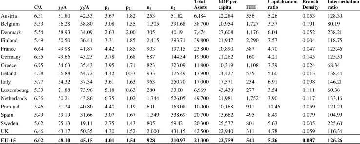
Table 1 provides summary statistics of the variables used in this study for the
overall sample and by country over the period 1998-2005. Comparing mean values
across countries, we can observe significant variations regarding total cost, outputs
and input prices, as well as country-level variables. In particular, the average cost to
assets ratio for all EU-15 countries stands at about 6 percent, ranging from 4.28
percent in Ireland to 6.75 percent in Greece. This indicates that there is still room for
improvement in terms of operating cost. Nevertheless, the average cost ratio for the
whole EU-15 region and for most EU member states follows a negative path over
time, in particular since 2001, flagging out banks’ efforts to restrain their cost
exposure. Moreover, the introduction of organizational changes (e.g. outsourcing), the
centralization of information technology and back-office activities and the
establishment of unified platforms appear to be widely applied strategies aiming at
reducing cost, standardizing operating and information procedures and exploiting
specialization according to the customer segment (ECB 2003).
(Please insert Table 1 about here)
assumption of risk neutrality for banks. 6
Substantial differences across the banking industry are also revealed by
looking at banks’ output structure in the respective European countries. Regarding
bank outputs, loans still comprise the largest proportion of banks’ balance sheets. In
detail, the average loans to assets ratio stands at about 48 percent, which is higher
than the average ratio of other earning assets, standing at about 45 percent.
Nevertheless, the increasing ratio of non-loan assets in banks’ balance sheets confirms
the trend of reorienting banking activities from traditional bank lending towards
investment activities, such as creating and selling new capital market products. We
should note, however, that in the majority of EU-15 countries, the loan ratio remains
higher than the other earning assets ratio, with the exception of Belgium, Ireland,
Luxembourg and the UK. Regarding input prices, note that the average price of
deposits stands at about 4 percent for the whole EU-15 region, ranging from 2.63 in
Denmark to 6.75 in Netherlands, while the average price of labour is 1.54, and ranges
from 0.37 in Ireland to about 2 percent in Denmark.
Country-level variables that capture the structure and regulatory environment
of banking markets also exhibit significant variation across EU member states.
Overall, it appears that the EU-15 banking industry is relatively unconcentrated,
although the Herfindahl index exhibits a fair amount of dispersion across EU-15
countries. Concentration is closely related to market size, as some of the smaller
countries tend to have a higher degree of concentration due to the presence of a few
large banks. This may point towards the presence of scale economies, since in a
smaller market fewer banks may be able to reach a viable size, whereas in a large
market, a smaller percentage share may provide sufficient scale to operate efficiently
(ECB 2004). Branch density also exhibits wide variation across countries, ranging
from 0.04 branches per square kilometre in Finland to 0.145 in Germany. This is also
the case for the capitalization ratio and for the average intermediation ratio, the latter
ranging from about 60 percent in Luxembourg to over 238 in Denmark.
4. Empirical Results
4.1. Inefficiency scores
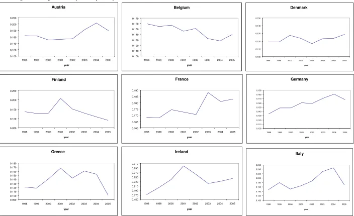
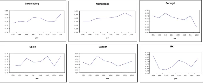
The average cost inefficiency scores per country and over time are presented
in Diagram 1.7 Our results are in line with the vast majority of the literature that
estimates the average cost inefficiency of EU countries in the range of 0.15 to 0.20
(see for example Allen and Rai 1996; Cavallo and Rossi 2001; Bos and Schmiedel
2003; Casu and Girardone 2004; Maudos and Guevara 2007). In particular, the
average cost inefficiency level for all EU-15 countries is estimated at 0.166, ranging
from 0.123 in Denmark to 0.237 in Ireland. The Scandinavian banking markets
(Denmark, Finland and Sweden) show remarkably low inefficiencies scores. Swedish
banks tend to be measured as best performers, despite the fact that these banks
suffered a crisis in the early 1990s requiring substantial government intervention
(Berger et al., 2000). On the other hand, countries that show a less rosy picture over
time are: Netherlands, Italy, France and the UK. The low performance in terms of
efficiency of the Italian and French banks could be partly explained by the slow pace
of deregulation that raises obstacles to improve operation based on new technologies
(Bikker 2002). In the case of the UK, though a country with an advanced financial
7
system, it ranks low in terms of cost efficiency in many efficiency studies (i.e.,
Altunbas et al. 2001; Cavallo and Rossi 2001; Casu and Girardone 2004), which
could be attributed to a low degree of competition.
(Please insert Diagram 1 about here)
Regarding the evolution of inefficiency scores over time, we observe different
patterns across countries. The highest improvement in terms of efficiency is observed
in Finland and Portugal, and to a lesser extent in Belgium. Late in the sample period a
sharp reduction of inefficiency is also observed in the case of Greece. Remarkably,
the underlying efficiency trends do not appear to show a common pattern across
EU-15, as Ireland, Luxembourg, Germany and Spain present a clear upward trend in
inefficiency over the examined period. In addition, we observe that the efficiency gap,
roughly measured as the difference between the most and the least cost efficient
banking sector, seems to have widened over time. In detail, the efficiency gap
increases significantly from 1998 to 2001, while it follows a diminishing pattern up to
2003. However, this trend is short-lived, as it is reversed after 2003.
The above results clearly demonstrate the existence of some diversity across
EU-15 countries given that no apparent homogenous pattern of inefficiency scores is
reported. This lack of homogeneity may reflect inherent differences in the underlying
markets due to historical differences in market structures, bank supervision,
regulation, legal traditions and due to different approaches that have been followed in
terms of the timing and the implementation of banking reforms. At a general level,
previous studies (Beck et al. 2003a,b; Beck and Levine 2004; La Porta et al. 1997,
1998; Levine 2003, 2004; Levine et al. 2000; Stulz and Williamson 2003) argue that
by differences in the legal tradition, the accounting conventions, the regulatory
structures, the property rights, the culture and even in the religion explain.
Despite the observed heterogeneity in the reported inefficiency levels, an
efficiency analysis fails to identify differences in the speed of reaction to a shock in
the short term. As a way of tackling this issue, we employ the quadratic loss function
that could provide evidence on convergence, if any, in the speed of adjustment
towards long-run equilibrium. If Europe’s banking markets have become more alike
over the eight-year period under consideration, we would expect to observe
convergence in the speed of adjustment across countries
4.2. Speed of adjustment across countries
Next, we employ the GMM estimator for dynamic panel data models proposed
by Arellano and Bond (1991) so as to estimate Equation (7), which includes the
lagged dependent variable (Cit-1) as an endogenous explanatory variable.8 Based on
Arellano and Bond (1991), we take first difference of Equation (7) on both sides and
remove in this way the firm-specific effects. The lagged dependent variables with
two or more periods are likely to be valid instruments for the equation in the first
differences, depending on whether disturbance it is serially correlated.9
8
The least squares estimator of the fixed effects or random effects models in the presence of a lagged dependent variable among the regressors is both biased and inconsistent (see for example, Baltagi 2001).
9
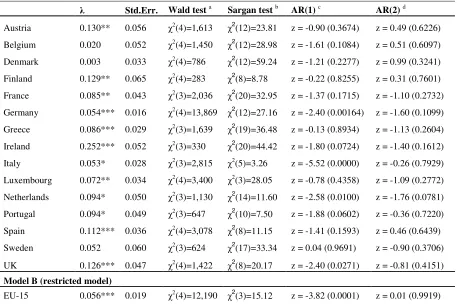
Table 2 presents the estimated results for our sample and reports some relevant
diagnostic tests.10 In our first unrestricted model (Model A), we estimate a different
persistent parameter for each country, in order to compare the speed of adjustment
across banking markets. In effect, identifies the persistence to a given level of
inefficiency, whereas 1- captures the adjustment speed to the long-run equilibrium.
takes values form 0 to 1, whereas the longer the current suboptimal inefficiency level
persists, the higher the value of . In this framework, if integration is occurring, we
would expect institutions from every country to ‘catch up’ with best practice and
therefore move towards a common EU-15 banking stochastic frontier at a higher
speed. Thus, a higher value of 1- would imply a higher degree of integration across
EU-15, as banks adjust their cost levels in a timelier manner so as to operate
efficiently in an increasingly competitive environment.
(Please insert Table 2 about here)
Table 2 shows that most of the persistent parameters are statistically
significant, but for Belgium, Denmark, and Sweden.11 Overall, we observe a
substantial variation in the estimated coefficients of across countries. In particular,
the estimates range from 0.053 in Italy to 0.25 in Ireland. This indicates that the
adjustment speed lies between 0.75 in Ireland and 0.95 in Italy. Thus, an Italian bank
is able to adjust its previous period’s inefficiency level at a much higher rate than an
Irish bank. In detail, the Italian banking industry has the highest adjustment speed
across EU countries, closely followed by Germany and Luxembourg. Although Italian
10
banks rank low in terms of cost efficiency, their ability to adjust their cost levels to
the long-run equilibrium in a timely manner indicates a ‘catching up’ process that
fosters integration. The high speed of adjustment observed in the Italian banking
industry, which ranks at the top of our country-list, could be the result of large-scale
consolidation and competitive pressure from other European countries. Similarly, the
good performance of German financial institutions could be the result of their
successful efforts to reduce their costs on a permanent basis and could also be
attributed to the three-pillar structure of the German banking system, which has
shown a high degree of flexibility and stability over the years. In a similar vein, the
high speed of adjustment in Luxembourg could be explained by the large presence of
foreign investors in the country.
Note that besides the slow speed of adjustment of Ireland, the speed of
adjustment is also relatively low in Austria, Finland, Spain and the UK, as indicated
by their high persistence parameters. Overall, we should also note that the average
level of inefficiency in each country appears to exhibit some relation to the speed of
adjustment towards equilibrium. In particular, the low speed of adjustment for Ireland,
Austria and the UK, all ranking low in terms of efficiency, suggests that their
“efficiency gap” with the best performers within EU not only has not narrowed over
time, but in contrast it has exhibited a positive trend. Undoubtedly, the widening of
“efficiency gap” does little to assist the European financial integration. On the other
hand, the low adjustment speed observed in the case for Finland, and to some extent
in the case of Spain, is less worrying for financial integration, as these banking
systems rank high in terms of efficiency.
11
The speed of adjustment in France, Greece, the Netherlands and Portugal takes
values that lie around the EU-15 average. In particular, the consolidation phase in the
French banking industry in the mid 90s, the privatization of state-owned credit
institutions that led to a drastic decrease in the number of bank branches and
employees in Greece and paved the way for greater profitability and efficiency, and
the liberalisation and increased competition in the Portuguese banking market along
with strong investment in information technology may have positively contributed to
an adequate speed of adjustment.
For comparison purposes, we also estimate a restricted model by imposing the
single adjustment speed restriction, i.e., letting c= for all countries. The single
persistence parameter by Model B is found to be quite low at 0.056. However, this
result must be treated with caution given that most of the country specific parameters
in Model A are significant. Thus, the imposition of c= for all countries on Model B
might appear too restrictive.
Overall, we observe significant differences in the estimated persistence
parameters across countries. The different speed of adjustment across banking
systems could reflect differences in the terms of institutions, supervisory rules,
government inferences, customer preferences and level of development across
countries. Moreover, differences in competitive conditions that affect the need to
reduce cost and to increase efficiency may explain the reported variation across
EU-15. Nevertheless, the relationship between the speed of adjustment towards
equilibrium and the average level of inefficiency in each banking industry is less
worst performer in terms of adjustment speed. On the other hand, Finland, which is
considered to be among the most efficient banking systems in the EU, appears to
adjust its costs to long-run equilibrium at a lower speed than the average.
4.3. Speed of adjustment over time
Next in our analysis, we investigate whether the adjustment speed changes
over the examined period. In order to do so and given data availability issues, we split
our sample into two sub-periods 1998-2001 and 2002-2005. If, indeed, the process of
integrating European banking markets increases competition, we would expect a
higher speed of adjustment over time. The estimated results are presented in Table
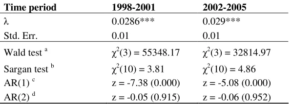
3.12 We observe that the persistent parameter is estimated at 2.8% for the sub-period
1998-2001, while it marginally increases at 2.9% for the period 2002-2005. Our
findings suggest that the adjustment speed has remained almost stable over the
examined period, though we can observe a slight decreasing trend between the two
periods from 97.2 to 97.1. A possible explanation could be that the first sub-period
coincides with a phase of an intense consolidation process in most banking systems,
swift rationalization of banks’ operations and increasing competition resulting from
the entry of new investors in most financial sectors. These developments could have
clearly improved banks’ performance and homogeneity across EU for the period
1998-2001, thereby leading to a somewhat lower adjustment speed for 2002-2005.
(Please insert Table 3 about here)
12
As a result, it appears at a first sight that the launch of the euro in 2002, along
with the intensifying efforts to achieve a higher degree of financial integrations have
not had a crucial impact, at least so far, on the speed of adjustment of banks.
5.
Conclusion
This paper provides insights on the issue of European integration by
examining the homogeneity across banking systems in terms of their underlying
adjustment speed of cost inefficiency to long-run equilibrium. In particular, we
employ a specification of a quadratic loss function based on forward-looking rational
expectations to model the underlying dynamics of total costs in the banking industry
of the EU-15 countries over the period 1998-2005. Based on this specification, for a
financial integration to occur, one would expect institutions from every country to
‘catch up’ with the best practice at a common speed. In particular, this paper shows
that the speed of adjustment is crucial for banking integration given the heterogeneity
observed in inefficiency scores across countries.
Our results indicate some differences in the adjustment speed across countries,
which could deter banking integration and could reflect, based on a recent paper by
the Sørensen and Gutiérrez (2006), the existence of inherent barriers to cross-border
trade in European banking and obstacles to the promotion of cross-country
competition. Different tax regimes on retail savings, limitations on cross-border
marketing of financial services, limits to hostile and cross-border takeovers in the
financial services industry in general, are among the possible factors that encourage
Gutiérrez 2006). Moreover, regarding the evolution of adjustment speed over time,
our findings suggest that the launch of the euro in 2002, along with the intensifying
efforts to achieve a higher degree of financial integration did not have an impact to
this day.
Overall, our analysis verifies the general notion that in retail banking, an area,
which is the most visible banking activity for customers, integration seems less
advanced than in other banking market segments such as wholesale and investment
banking, as it is evident from the present reported heterogeneity in inefficiency levels,
and in the speed of adjustment towards equilibrium across countries. These results
suggest that banks, on average, could accelerate further the pace of adjustment of their
cost efficiency over time, also in light of the ongoing global financial harmonization
and liberalization. In response to growing domestic and international competitive
pressures, banks are bound to further enhance their performance by minimizing their
operation costs at a higher speed, employing optimal production plans, adopting new
technologies, and reducing excess capacity through mergers. Since only the most
efficient institutions will survive these challenges, the inefficient banks with a slow
adjustment pace will either be acquired or eventually be driven out of market by the
competition.
For this reason, it is of particular interest for policy makers, regulatory
authorities and expert practitioners alike to have accurate information about the true
underlying differences in bank performance among European countries so as to adjust
to a highly evolving new and globalized environment, to undertake strategic
increasing competition in domestic as well as cross-border markets (Barros et al.
2007). A policy proposal for bank managers so as to raise the speed of adjustment is
to employ a flexible cost structure. In addition, the challenge for policy makers is to
avoid complacency and to continue addressing the structural weaknesses that are still
holding back European banking integration and limit the EU capacity to make the
most of a single banking market. Nevertheless, quoting Padoa-Schioppa (2005):
‘political and regulatory bodies have to create the framework for financial
integration but it is up to market forces to exploit this potential’. Yet, the European
financial integration provides an opportunity to accelerate structural reform efforts in
References
Aigner, D.J., Lovell, C.A.K., Schmidt, P.1977. “Formulation and estimation of stochastic frontier production function models,” Journal of Econometrics 6(1), 21-37.
Allen, L. Rai, A.1996. “Operational efficiency in banking: an international comparison,” Journal of Banking and Finance 20, 655-672.
Altunbas, Y., Gardener, E.P.M., Molyneux, P., Moore, B.2001. “Efficiency in European banking,” European Economic Review 45 (10), 1931–1955.
Arellano, M., Bond, S. R.1991. “Some tests of specification for panel data: Monte Carlo evidence and an application to employment equations,” Review of Economic Studies 58, 277-297.
Baele, L., Ferrando, A., Hördahl, P., Krylova, E., Monnet, C.2004. “Measuring Financial Integration in the euro area,” Occasional Paper Series No. 14, European Central Bank.
Baltagi, B.H. 2001. “Econometric Analysis of Panel Data (2nd edition),” John Wiley & Sons, Chichester.
Barros, C.P., Ferreira, C., Williams, J.2007. “Analysing the determinants of
performance of best and worst European banks: A mixed logit approach,” Journal of Banking and Finance 31, 2189–2203.
Beck, T., Levine, R.2004. “Stock markets, banks and growth: Panel evidence,” Journal of Banking and Finance 28, 423–442.
Beck, T., Demirguc-Kunt, A., Levine, R. 2003a. “Law, endowments, and finance,” Journal of Financial Economics 70, 137–181.
Beck, T., Demirguc-Kunt, A., Levine, R. 2003b. “Law and finance. Why does legal origin matter?” Journal of Comparative Economics 31, 653–675.
Berger, A.N., Dai, Q., Ongena, S., Smith, D. 2003. “To what extent will the banking system become globalized?” A study of bank nationality and reach in 20
European countries. Journal of Banking and Finance 27, 383–415.
Berger, A.N., DeYoung, R., Genay, H., Udell, G.F. 2000. “The globalization of financial institutions: Evidence from cross-border banking performance,” Brookings-Wharton Papers on Financial Services 3, 23–158.
Berger, A.N., De Young, R., Udell, G. 2001. “Efficiency barriers to the consolidation of the European financial services industry,” European Financial Management 7, 117–130.
Berger, A.N., Mester, L.J.1997. “Inside the black box: what explains differences in the efficiencies of financial institutions?” Journal of Banking and Finance 21(7), 895-947.
Bikker, J.A. 2002. “Efficiency and cost differences across countries in a unified banking market,” Kredit und Kapital 35, 344–380.
Bos, J.W.B., Schmiedel, H. 2003. “Comparing efficiency in European banking: a meta frontier approach,” Research Series Supervision no. 57, Directorate Supervision, De Nederlandische Bank.
Buch, C.M., Heinrich, R.P. 2002. “Financial integration in Europe and banking sector performance,” Kiel Institute of World Economics, Mimeo.
Cabral, I., Dierick, F., Vesala, J. 2002. “Banking integration in the euro area,” Occasional Paper Series No. 6, European Central Bank.
Cappiello, L., Hordahl, P., Kadareja, A., Manganelli, S.2006. “The impact of the euro on financial markets,” ECB Working Paper no. 598.
Casu, B., Girardone, C.2004. “Large banks’ efficiency in the single European market,” The Service Industries Journal 24(6), 129–142.
Casu, B., Girardone, C. 2006. “Bank competition, concentration and efficiency in the Single European banking market,” The Manchester School 74(4), 441-468.
Casu, B., Molyneux, P. 2003. “A comparative study of efficiency in European banking,” Applied Economics 35(17), 1865-1876.
Cavallo, L., Rossi, S.P.S.: Scale and scope economies in the European banking systems. Journal of Multinational Financial Management 11, 515–531 (2001).
Cuthbertson, K., Taylor, M.P. 1990. “Money demand, expectations and the forward-looking model,” Journal of Policy Modeling 12, 289-315.
De Guevara, J.F., Maudos, J. 2002. “Inequalities in the efficiency of the banking sectors of the European Union,” Applied Economics Letters 9, 541-544.
Demsetz, H. 1973. “Industry structure, market rivalry and pubic policy,” Journal of Law and Economics 16, 1-9.
Dietsch, M., Lozano-Vivas, A. 2000. “How the environment determines banking efficiency: a comparison between French and Spanish industries,” Journal of Banking and Finance 24, 985-1004.
Emiris, M. 2002. “Measuring capital market integration,” BIS Papers 12, 200–221.
European Central Bank. 2000. “Mergers and Acquisitions Involving the EU Banking Industry: Facts and Implications,” December. ECB, Frankfurt.
European Central Bank. 2003. “Structural analysis of the EU banking sector: Year 2002,” ECB, November.
European Central Bank. 2004. “Report on EU banking structure,” ECB, November.
European Commission. 2001. “Financial market integration in the EU,” Chapter IV, EU Economy Review, DG ECFIN.
Freixas, X. 2003. “European banking integration: where do we stand?” Deutsche Bank Lecture, Saıd Business School, Oxford.
Goddard, J. Molyneux, P., Wilson, J.O.S., Tavakoli, M. 2007. “European Banking: an overview,” Journal of Banking and Finance 31, 1911–1935.
Guiso, L., Jappelli, T., Padula, M., Pagano. M. 2004. “Financial market integration and economic growth in the EU,” Economic Policy, 523–577.
Hartmann, P., Maddaloni, A., Manganelli, S. 2003. “The euro area financial system: Structure, integration and policy,” Oxford Review of Economic Policy 19, 180– 213.
Heinemann, F., Jopp, M. 2002. “The benefits of a working European retail market for EU financial service,”. Institut fur Europaische Politik, Berlin.
Huang, T.H., Chen, W.H. 2006. “A study on long run inefficiency levels of a panel dynamic cost frontier under the framework of forward-looking rational
expectations” Mimeo.
Huang, T.H., Shen, C.H. 2002. “Seasonal cointegration and cross-equation
restrictions on a forward-looking buffer stock model of money demand,” Journal of Econometrics 111, 11-46.
Hughes, J.P., Lang, W., Mester, L.J., Moon, C. 1996. “Efficient banking under interstate branching,” Journal of Money Credit Banking28, 1045–1071.
Hughes, J., Moon, C. 1995. “Measuring bank efficiency when managers trade return for reduced risk,” Working Paper, Department of Economics, Rutgers University.
Jondrow, J., Lovell, C.A.K. Materov, I., Schmidt, P. 1982 “On the estimation of technical inefficiency in the stochastic frontier production model,” Journal of Econometrics 19(2/3), 233-238.
La Porta, R., Lopez-de-Silanes, F., Shleifer, A., Vishny, R. 1997. “Legal determinants of external finance.” Journal of Finance 52, 1131–1150.
Levine, R. 2003. “Bank-based or market-based financial systems: Which is better?” Journal of Financial Intermediation 11, 398–428.
Levine, R. 2004. “Finance and growth: Theory and evidence,” NBER Working Paper No. 10766.
Levine, R., Loayza, N., Beck, T. 2000. “Financial intermediation and growth: causality and causes,” Journal of Monetary Economics 46, 31–77.
Lozano-Vivas, A., Pastor, J.T., Hasan, I. 2001. “European bank performance beyond country borders: what really matters?” European Finance Review 5, 141–165.
Lozano-Vivas, A., Pastor, J.T., Pastor, J.M. 2002. “An efficiency comparison of European banking systems operating under different environmental conditions,” Journal of Productivity Analysis 18, 59–77.
Manna, M. 2004. “Developing statistical indicators of the integration of the euro area banking system,” ECB working paper no. 300.
Maudos, J., De Guevara, J.F. 2007. “The cost of market power in banking: social welfare loss vs. cost inefficiency,” Journal of Banking and Finance 31, 2103– 2125.
Maudos, J. Pastor, J.M., Perez, F. 2002. “Quesada, J.: Cost and profit efficiency in European banks,” Journal of International Financial Markets, Institutions and Money 12, 33–58.
Meeusen, W., van den Broeck, J. 1997. “Efficiency estimation from Cobb-Douglas production functions with composed error,” International Economic Review 18(2), 435-444.
Mester, L. J. 1996. “A study of bank efficiency taking into account risk-preferences,” Journal of Banking and Finance 20, 1025-1045.
Mizen, P.D. 1994. “A buffer stock model of the demand for money for the personal sector,” Bulletin of Economic Research, 46, 289-314.
Molyneux, P., Altunbas, Y., Gardener, E. 1977 “Efficiency in European Banking,” John Wiley & Sons, West Sussex, UK.
Padoa-Schioppa, T. 2005. “Introductory Speech: Germany and European Financial Integration,” Conference Proceedings: Open Forum on Germany’s banking system, Center for Financial Studies at the University of Frankfurt.
Schuler, M., Heinemann, F. 2002. “How integrated are European retail financial markets? A cointegration analysis,” Centre for European Economic Research (ZEW), Mimeo.
Sørensen, C.K., J.M. Gutiérrez. 2006 “Euro area banking sector integration using hierarchical cluster analysis techniques,” Working Paper Series No 627, European Central Bank.
Stulz, R., Williamson, R.2003. “Culture, openness, and finance” Journal of Financial Economics 70, 313–349.
Table 1: Summary Statistics (pooled sample 1998-2005)
C/A y1/A y2/A p1 p2 n1 n2
Total Assets
GDP per
capita HHI
Capitalization ratio
Branch Density
Intermediation ratio
Austria 6.31 51.80 42.53 3.67 1.82 253 51.82 6,184 22,284 556 5.26 0.053 128.30
Belgium 5.53 36.28 58.80 3.08 1.55 1,305 391.68 38,700 20,954 1,727 3.37 0.191 80.19
Denmark 5.54 58.93 34.09 2.63 2.00 305 40.19 7,474 27,608 1,176 6.04 0.052 238.21
Finland 5.49 50.50 36.41 3.31 1.85 2,415 393.71 39,800 21,947 2,290 7.57 0.004 118.75
France 6.64 49.98 41.87 4.42 1.85 903 197.15 23,800 20,890 587 4.70 0.047 123.46
Germany 6.35 49.66 45.23 3.78 1.68 687 144.54 19,900 21,262 160 4.21 0.145 125.50
Greece 6.75 54.63 35.43 3.95 1.71 823 323.09 11,800 10,319 1,108 7.39 0.024 68.34
Ireland 4.28 36.88 54.72 4.42 0.37 933 125.49 17,900 24,427 535 5.60 0.013 138.44
Italy 5.77 54.32 37.34 3.61 1.63 963 250.70 17,000 17,571 234 6.91 0.098 146.21
Luxembourg 5.33 21.88 73.96 5.18 0.63 280 33.00 6,969 43,439 277 3.54 0.111 60.38
Netherlands 6.36 50.21 43.86 6.75 1.02 1,744 526.05 49,700 21,981 1,752 3.90 0.117 133.16
Portugal 5.46 51.24 40.80 4.40 1.19 691 163.08 10,900 10,168 911 10.46 0.059 121.29
Spain 5.49 59.19 31.66 3.07 1.67 1,349 338.69 20,700 13,662 495 8.49 0.079 104.99
Sweden 5.02 75.13 19.11 2.75 1.43 805 59.42 20,300 25,577 801 5.63 0.005 225.60
UK 6.46 43.17 50.35 4.30 1.52 2,000 431.15 42,500 22,940 311 4.78 0.059 116.34
EU-15 6.02 48.10 45.15 4.01 1.54 928 210.97 21,300 22,759 541 5.26 0.087 126.26
Figure 1: Average Inefficiency scores by country
Note: The above graphs present the average cost inefficiency scores for each country and their evolution over time, as derived from a common stochastic cost frontier, where Log likelihood function=311.94; 2v=0.027; 2u= 0.084; =Sqr[ 2v+ 2u]=0.331. Mean inefficiency=0.166. Inefficiency is assumed to follow an exponential distribution and ranges between zero and unity.
Italy 0.100 0.120 0.140 0.160 0.180 0.200 0.220 0.240 0.260
1998 1999 2000 2001 2002 2003 2004 2005
year Ireland 0.150 0.170 0.190 0.210 0.230 0.250 0.270 0.290 0.310
1998 1999 2000 2001 2002 2003 2004 2005 year Austria 0.100 0.120 0.140 0.160 0.180 0.200 0.220
1998 1999 2000 2001 2002 2003 2004 2005 year Belgium 0.100 0.110 0.120 0.130 0.140 0.150 0.160 0.170
1998 1999 2000 2001 2002 2003 2004 2005 year Denmark 0.100 0.110 0.120 0.130 0.140 0.150
1998 1999 2000 2001 2002 2003 2004 2005
year Finland 0.050 0.100 0.150 0.200 0.250
1998 1999 2000 2001 2002 2003 2004 2005 year France 0.160 0.165 0.170 0.175 0.180 0.185 0.190
1998 1999 2000 2001 2002 2003 2004 2005 year Germany 0.100 0.110 0.120 0.130 0.140 0.150 0.160 0.170 0.180 0.190
1998 1999 2000 2001 2002 2003 2004 2005
year Greece 0.090 0.100 0.110 0.120 0.130 0.140 0.150 0.160 0.170 0.180
Figure 1 (continued) UK 0.150 0.155 0.160 0.165 0.170 0.175 0.180 0.185 0.190 0.195
1998 1999 2000 2001 2002 2003 2004 2005 year Portugal 0.080 0.090 0.100 0.110 0.120 0.130 0.140 0.150 0.160
1998 1999 2000 2001 2002 2003 2004 2005 year Luxembourg 0.100 0.120 0.140 0.160 0.180 0.200 0.220
1998 1999 2000 2001 2002 2003 2004 2005 year Netherlands 0.100 0.120 0.140 0.160 0.180 0.200 0.220
1998 1999 2000 2001 2002 2003 2004 2005 year Spain 0.100 0.110 0.120 0.130 0.140 0.150 0.160 0.170
1998 1999 2000 2001 2002 2003 2004 2005 year Sweden 0.090 0.100 0.110 0.120 0.130 0.140 0.150 0.160
[image:31.792.44.751.68.358.2]Table 2: Estimates of persistence parameter for each country
Model A (unrestricted model)
Std.Err. Wald test a Sargan test b AR(1) c AR(2) d
Austria 0.130** 0.056 2(4)=1,613 2(12)=23.81 z = -0.90 (0.3674) z = 0.49 (0.6226)
Belgium 0.020 0.052 2(4)=1,450 2(12)=28.98 z = -1.61 (0.1084) z = 0.51 (0.6097)
Denmark 0.003 0.033 2(4)=786 2(12)=59.24 z = -1.21 (0.2277) z = 0.99 (0.3241)
Finland 0.129** 0.065 2(4)=283 2(8)=8.78 z = -0.22 (0.8255) z = 0.31 (0.7601)
France 0.085** 0.043 2(3)=2,036 2(20)=32.95 z = -1.37 (0.1715) z = -1.10 (0.2732)
Germany 0.054*** 0.016 2(4)=13,869 2(12)=27.16 z = -2.40 (0.00164) z = -1.60 (0.1099)
Greece 0.086*** 0.029 2(3)=1,639 2
(19)=36.48 z = -0.13 (0.8934) z = -1.13 (0.2604)
Ireland 0.252*** 0.052 2(3)=330 2(20)=44.42 z = -1.80 (0.0724) z = -1.40 (0.1612)
Italy 0.053* 0.028 2(3)=2,815 2(5)=3.26 z = -5.52 (0.0000) z = -0.26 (0.7929)
Luxembourg 0.072** 0.034 2(4)=3,400 2(3)=28.05 z = -0.78 (0.4358) z = -1.09 (0.2772)
Netherlands 0.094* 0.050 2(3)=1,130 2(14)=11.60 z = -2.58 (0.0100) z = -1.76 (0.0781)
Portugal 0.094* 0.049 2(3)=647 2
(10)=7.50 z = -1.88 (0.0602) z = -0.36 (0.7220)
Spain 0.112*** 0.036 2(4)=3,078 2(8)=11.15 z = -1.41 (0.1593) z = 0.46 (0.6439)
Sweden 0.052 0.060 2(3)=624 2(17)=33.34 z = 0.04 (0.9691) z = -0.90 (0.3706)
UK 0.126*** 0.047 2(4)=1,422 2(8)=20.17 z = -2.40 (0.0271) z = -0.81 (0.4151)
Model B (restricted model)
EU-15 0.056*** 0.019 2(4)=12,190 2(3)=15.12 z = -3.82 (0.0001) z = 0.01 (0.9919)
Note: ***, ** and * indicate 1%, 5% and 10% significance levels, respectively. Model A is the unrestricted model, with separate persistent parameters ( ) for each country; Model B is the restricted model, with a common persistent parameter for all EU-15 countries. The speed of adjustment is defined as 1- .
a
:Wald statistic is a test for the joint significance of the independent variables asymptotically distributed as 2(k) under the null hypothesis of no relationship, where K denotes the number of slope coefficients estimated.
b
: Sargan test is the test for over-identifying restrictions in GMM dynamic model estimation. c
: Arellano-Bond test that average autocovariance in residuals of order 1 is 0 (H0: No autocorrelation). p-values in parentheses.
d
Table 3: Estimates of persistence parameter over time
Time period 1998-2001 2002-2005
0.0286*** 0.029***
Std. Err. 0.01 0.01
Wald test a 2(3) = 55348.17 2(3) = 32814.97
Sargan test b 2(10) = 3.81 2(10) = 4.86 AR(1) c z = -7.38 (0.000) z = -5.08 (0.000) AR(2) d z = -0.05 (0.915) z = -0.06 (0.952)
Note: *** and * indicate 1% and 10% significance levels, respectively. We estimated separate dynamic regressions for each sub-period and for each type of ownership. The speed of adjustment is defined as 1- .
a:Wald statistic is a test for the joint significance of the independent variables
asymptotically distributed as 2(k) under the null hypothesis of no relationship, where K denotes the number of slope coefficients estimated.
b
: Sargan test is the test for over-identifying restrictions in GMM dynamic model estimation.
c
: Arellano-Bond test that average autocovariance in residuals of order 1 is 0 (H0: No autocorrelation). p-values in parentheses.
d