Munich Personal RePEc Archive
Bandwidth selection for continuous-time
Markov processes
Bandi, Federico and Corradi, Valentina and Moloche,
Guillermo
Johns Hopkins University Carey Business School, University of
Chicago Booth School of Business, Warwick University, University of
Chicago, Pontificia Universidad Católica del Perú
30 October 2009
Online at
https://mpra.ub.uni-muenchen.de/43682/
Bandwidth Selection for Continuous-Time Markov Processes
Federico M. Bandi, Valentina Corradi, and Guillermo Moloche
Johns Hopkins University, University of Warwick, and University of Chicago October 2009
Abstract
We propose a theoretical approach to bandwidth choice for continuous-time Markov processes. We do so in the context of stationary and nonstationary processes of the recurrent kind. The procedure consists of two steps. In the …rst step, by invoking local Gaussianity, we suggest an automated band-width selection method which maximizes the probability that the standardized data are a collection of normal draws. In the case of di¤usions, for instance, this procedure selects a bandwidth which only ensures consistency of the in…nitesimal variance estimator, not of the drift estimator. Addi-tionally, the procedure does not guarantee that the rate conditions for asymptotic normality of the in…nitesimal variance estimator are satis…ed. In the second step, we propose tests of the hypothesis that the bandwidth(s) are either "too small" or "too big" to satisfyall necessary rate conditions for consistency and asymptotic normality. The suggested statistics rely on a randomized procedure based on the idea of conditional inference. Importantly, if the null is rejected, then the …rst-stage band-widths are kept. Otherwise, the outcomes of the tests indicate whether larger or smaller bandband-widths should be selected. We study scalar and multivariate di¤usion processes, jump-di¤usion processes, as well as processes measured with error as is the case, for instance, for stochastic volatility modelling by virtue of preliminary high-frequency spot variance estimates. The …nite sample joint behavior of our proposed automated bandwidth selection method, as well as that of the associated (second-step) randomized procedure, are studied via Monte Carlo simulation.
Keywords: Bandwidth selection, recurrence, Continuous-time Markov processes.
1
Introduction
Following in‡uential, early work on fully nonparametric in…nitesimal volatility estimation and testing for scalar di¤usion processes (e.g., Brugiére, 1991, Corradi and White, 1999, Florens-Zmirou, 1993, and Jacod 1997), the recent nonparametric literature in continuous time has largely focused on the full system. Emphasis might, for instance, be also placed on the estimation of the …rst in…nitesimal moment (the drift) in the di¤usion case (Stanton, 1997, among others) and, in the case of jump-di¤usions, on the high-order in…nitesimal moments (Johannes, 2004,inter alia).
Motivated by the need to completely characterize the system’s dynamics, Bandi and Phillips (2003) have established consistency and asymptotic (mixed) normality for Nadaraya-Watson kernel estimators of both the drift and the di¤usion function of recurrent (and, hence, possibly nonstationary) scalar di¤usion processes (see, also, Fan and Zhang, 2003, and Moloche, 2004, for local polynomial estimates under stationarity and recurrence, respectively). Their results rely on a double asymptotic design in which the interval between discretely-sampled observations approaches zero, in-…ll asymptotics, and the time span diverges to in…nity, long-span asymptotics. A signi…cant di¤erence between a stationary (or positive recurrent) di¤usion and a nonstationary (or null recurrent) one is that in the former case the local time grows linearly with the time span, while in the latter case it grows at a slower (and, generally, unknown) rate. Because the rate of divergence of local time a¤ects the rate of convergence of the functional estimates of the process moments, this observation is theoretically, and empirically, important. Bandi and Moloche (2004) have generalized the results in Bandi and Phillips (2003) to the case of multidimensional di¤usion processes. Importantly, in the multidimensional case a well-de…ned notion of local time no longer exists and one has to rely on the more general notion of occupation density. In both the scalar and the multidimensional case, consistency and (mixed) normality of the drift and variance estimator (and, hence, of the full system’s dynamics) rely on the proper choice of the bandwidth parameters, i.e., on the rate at which the bandwidths approach zero as the interval between discretely-sampled observations goes to zero and the corresponding occupation densities (or local times, in the scalar case) diverge to in…nity.
band-width selection has been made by Karlsen and Tjostheim (2001) for -null recurrent processes and by Guerre (2004) for general recurrent processes. The continuous-time case poses additional complications in that not only one has to adapt to the level of recurrence in the estimation domain but, also, to the rate at which the interval between discretely-sampled observations vanishes asymptotically.
This paper attempts to …ll this important gap in the continuous-time econometrics literature by proposing a theoretical approach to automated bandwidth choice. The approach is designed for widely-employed classes of continuous-time Markov processes, such as scalar and multivariate di¤usion processes and jump-di¤usion processes, and is justi…ed under mild assumptions on their statistical properties, stationarity not being required. Our solution to the problem is novel and may also be applied to discrete-time models, as outlined in Section 8.
In the di¤usion case, the intuition of our approach is as follows. Consider kernel estimates of drift and di¤usion function (bhdr andbhdif). Assume these estimates are obtained by selecting di¤erent smoothing
sequences. Invoking the local Gaussianity property which di¤usion models readily imply as a useful prior on the distributional feature of the standardized data, we maximize the probability that the standardized data (Xt+ Xt) bhdr(Xt)
bhdif(Xt)
p is a collection of draws from a Gaussian distribution by choosing the relevant
smoothing sequences (hdr andhdif) accordingly. This procedure selects a bandwidthhdif which ensures the consistency of the in…nitesimal variance estimator but, in spite of its sound empirical performance (see Section 7), does not select a bandwidthhdr which ensures the theoretical consistency of the drift function. Also, the automatically-chosen bandwidths do not necessarily satisfy the rate conditions required for (mean zero) asymptotic normality. To overcome this issue, for each in…nitesimal moment, we propose a test of the null hypothesis that one or more rate conditions (for consistency and normality) are violated versus the alternative that all rate conditions are satis…ed. The suggested statistics (separately speci…ed for drift and di¤usion) rely on a randomized procedure based on the idea of conditional inference, along the lines of Corradi and Swanson (2006). If the null is rejected, then the selected bandwidth is kept, otherwise the outcome of the procedure suggests whether we should select a larger or a smaller bandwidth. We proceed sequentially, until the null is rejected. Because the probability of rejecting the null when the it is false is asymptotically one at each step, our approach does not su¤er from a sequential bias problem.
We begin by considering the case of bandwidth selection for scalar di¤usion models (Section 2). We then extend our analysis to scalar jump-di¤usion processes (Section 3). The case of a di¤usion observed with error is presented in Section 4. Stochastic variance processes …ltered from high-frequency …nancial data may, of course, be regarded as processes observed with error. We evaluate the case of stochastic volatility explicitly and discuss bandwidth selection for di¤usion models applied to market microstructure noise-contaminated spot variance estimates in Section 5. In Section 6 we study the multivariate di¤usion case. Section 7 provides a Monte Carlo study. Section 8 contains …nal remarks. All proofs are collected in the Appendix.
2
Scalar di¤usion processes
2.1 The framework
We consider the following class of one-factor models,
dXt= (Xt)dt+ (Xt)dWt;
wherefWt:t= 1; :::; Tg is a standard Brownian motion. Our objective is to provide suitable nonpara-metric estimates of the drift term (a)and of the in…nitesimal variance 2(a):To this extent, we assume availability of a sample of N equidistant observations and denote the discrete interval between two successive observations as N;T = T =N, where T de…nes the time span. Speci…cally, we observe the di¤usion skeletonX N;T; X2 N;T; :::; XN N;T:In what follows, we requireN; T ! 1; N;T ! 0 (in-…ll
asymptotics), andT = N;TN ! 1 (long-span asymptotics) for consistency of the moment estimates. As in Stanton (1997), Bandi and Phillips (2003), and Johannes (2004), inter alia, we construct the following estimators of the drift and in…nitesimal variance, respectively:
bN;T(a) =
1
N;T
PN 1
j=1 K
Xj N;T a
hdr N;T
X(j+1) N;T Xj N;T
PN
j=1K
Xj N;T a
hdr N;T
; (1)
and
b2N;T(a) =
1
N;T
PN 1
j=1 K
Xj N;T a
hdifn;T X(j+1) N;T Xj N;T
2
PN
j=1K
Xj N;T a
hdifN;T
: (2)
We denote byh= hdr
N;T; hdifN;T 2H R2+a bivariate vector bandwidth belonging to the setHcontained
in the positive plane R2+. This vector is our object of econometric interest. Assumption 1 guarantees existence of a unique, recurrent solution to X. Assumption 2 outlines the conditions imposed on the kernel functionK(:)in Eqs. (1) and (2). The same conditions on the kernel function are also employed
Assumption 1.
(i) (:) and (:) are time-homogeneous, B-measurable functions on D= (l; u) with 1 l < u 1;
where B is the -…eld generated by Borel sets on D. Both functions are at least twice continuously di¤erentiable. Hence, they satisfy local Lipschitz and growth conditions. Thus, for every compact subset J of the range of the process, there exist constants C1J and C2J so that, for all x and y in J,
j (x) (y)j+j (x) (y)j C1Jjx yj; and
j (x)j+j (x)j C2Jf1 +jxjg.
(ii) 2(:)>0 on D.
(iii) We de…ne S( ), the natural scale function, as
S( ) =
Z
c
exp Z y
c
2 (x)
2(x) dx dy;
where cis a generic …xed number belonging to D. We require S( ) to satisfy
lim
!lS( ) = 1:
and
lim
!uS( ) =1:
Assumption 2. The kernel K(:)is a continuously di¤erentiable, symmetric and nonnegative function whose derivative K0(:) is absolutely integrable and for which
Z 1
1
K(s)ds= 1; K2 =
Z 1
1
K2(s)ds <1; sup
s K(s)< C3;
and
Z 1
1
s2K(s)ds <1:
In what follows, the symbol LX(T; a) denotes the chronological local time of X atT and a, i.e., the number of calendar time units spent by the process aroundain the time interval[0; T].
Proposition 1 (Bandi and Phillips, 2003): Let Assumptions 1 and 2 hold.
(i) Let N;T =T =N withT …xed. If limN!1hN;T1 N;Tlog 1
N;T
1=2
!0, then
b
LX(T ; a) LX(T ; a) =oa:s:(1); whereLbX(T ; a) = hN;T
N;T
PN
j=1K
Xj
N;T a
The drift estimator
Let (ii) hdr
N;TLX(T; a)a:s:! 1 and (iii) LXhdr(T;a) N;T N;T
log 1
N;T
1=2 a:s:
! 0;then:
bN;T(a) (a) =oa:s:(1): Further, if (iv) hdr;N;T5LX(T; a)a:s:! 0;then:
r
hdrN;TLbX(T; a) bN;T(a) (a) )N 0;K2 2(a) :
The di¤usion estimator
If (iii) holds with hdr
N;T replaced byhdifN;T, then:1
b2N;T(a) 2(a) =oa:s:(1):
Further, if (iv’) hdif;5N;T LX(T;a) N;T
a:s:
! 0;then:
v u u
thdifN;TLbX(T; a)
N;T b
2
N;T(a) 2(a) )N 0;2K2 4(a) :
It is evident from the proposition above (as well as classical logic based on nonparametric moment estimation in discrete time) that consistency and asymptotic normality of the drift and variance estimator crucially rely on appropriate choice of the smoothing parameter(s). To this extent, two issues ought to be addressed. First, usual data-driven methods often employed in empirical work in continuous-time …nance, such as cross-validation, are not theoretically justi…ed and may not necessarily work in the presence of in-…ll asymptotics and nonstationarity. Second, while in the positive recurrent caseLX(T; a)=T !p fX(a); where fX(a) denotes the stationary probability density at a of the process X; in the null recurrent case LX(T; a)=T
p
! 0. Under null recurrence, as emphasized earlier, LX(T; a) grows at a (generally unknown) rate which is slower thanT.2 Since the bandwidth’s vanishing rate depends on this unknown rate, appropriate bandwidth selection in the null recurrent case is particularly delicate.
We shall proceed in two steps. In the …rst step, we introduce an adaptive bandwidth selection method which ensures consistency of the di¤usion estimator but only guarantees that bN;T(a) (a) = op N;T1=2 : In the second step, we employ a randomized procedure to test whether the bandwidth selected in the …rst stage violate any of the rate conditions (ii)-(iii)-(iv) for the drift and (iii)-(iv’) for the di¤usion. This second step is conducted separately for drift and di¤usion. Should we reject the null, then we would rely on the previously-chosen bandwidth. Alternatively, because the outcome of the procedure gives us information about whether the selected bandwidth is too small or too large, we iterate until the null is rejected.
1Note that (iii) ensures that hdifN;TLbX(T;a)
N;T ! 1:
2The Brownian motion case is an exception for which the rate is known and L
X(T; a)=
p
2.2 First step: A residual-based procedure
Consider the estimated residual series
(
b"i N;T =
Xi N;T X(i 1) N;T bN;T(X(i 1) N;T) N;T
bN;T(X(i 1) N;T)
p
N;T
: i= 2; :::; N;T1 T
)
;
assuming, for notational simplicity, that 1
N;T is an integer. In light of the normality of the driving Brownian motion, over small time intervals N;T the residual series is roughly standard normally dis-tributed. Our minimization problem requires …nding
b
hN;T 2H R+2 : FbhN;T
N ; = N (3)
with N # 0 as N = N;T1 T ! 1, where FbhN;T
N denotes the empirical cumulative distribution of the estimated residuals b"i N;T, is the cumulative distribution of the standard normal random variable,
and (:; :) is a distance metric.
It is noted that the criterion is de…ned over a …xed time span T whereas the estimators, mainly for consistency of the drift, are de…ned over an enlarging span of time T: We de…ne the criterion over a …xed time span to avoid theoretical imbalances in the case of nonstationary di¤usions. This point is discussed in Bandi and Phillips (2007). From an empirical standpoint, …xing the sample span over which the criterion is minimized and enlarging the time span over which the nonparametric estimators are computed is immaterial. It simply amounts to splitting the sample into two parts, i.e. (0; T] and
(T ; T]. The entire sample (from 0 toT) is used to compute bN;T(:) and bN;T(:). The …rst part of the sample (from0 toT) is used to de…ne the minimization problem.3
We focus on the Kolmogorov-Smirnov distance, but a di¤erent distance measure may, of course, be employed. We de…ne the target bandwidth sequence h
N;T = (hdrN;T; h dif
N;T) as the bandwidth sequence which guarantees that the empirical distribution function of the standardized data converges uniformly to the standard normal distribution function as N; T ! 1 with NT ! 0 (and, of course, with N =
T N;T1 ! 1). We will …rst characterize its properties (in Theorem 1). Subsequently, we will show that it exists and thathbN;T is asymptotically equivalent to it (in Theorem 2).
Theorem 1. A vector bandwidth h
N;T = (hdrN;T; h dif
N;T) satis…es
h
N;T =h2H: sup
x
FNh(x) (x) !p
N;T!1; N;T!0
0 (4)
if and only if
3This statement can easily be reconciled with our theoretical framework. AssumeT =pN, for instance. Then, the observations are equispaced atnp1
N; 2
p
N; :::;1;1 + 1
p
N; :::;
p
Nosince T N =
1
p
N. We can now split the sample in
two parts, namely observations in(0; T]and observations in(T ; T]:Assume, without loss of generality, thatT = 1.
Also, assume that there are N equispaced observations in the …rst part of the sample. Then, 1 N =
1
p
N. This
sup
a2D bN;T
a; hdrN;T (a) =op p 1 N;T
!
; (5)
and
sup
a2D b
N;T a; hdifN;T (a) =op(1): (6)
Theorem 2. Let Assumptions 1 and 2 hold. (i)There exists a vector bandwidth h
N;T = (hdrN;T; h dif N;T)
so that
hN;T =h2H: sup
x F
h
N(x) (x)
p
!
N;T!1; N;T!0
0 (7)
and
h
N;T = hdrN;T; hdifN;T N;T!1!;
N;T!0
0: (ii)If
b
hN;T =h2H: sup
x F
h
N(x) (x) = N (8)
with N #0as N ! 1,then
b
hN;T=hN;T !p
N;T!1; N;T!0
1:
Theorem 2 guarantees the existence of a bandwidth vectorhbN;T ensuring that our proposed criterion
has a solution. This solution guarantees uniform consistency (in probability) of the variance estimator but, despite being empirically very sensible as we show below through simulations (see Section 7), fails to guarantee theoretical consistency of the drift estimator. In addition, the selected di¤usion bandwidth does not ensure asymptotic normality of the di¤usion estimator. A second procedure is therefore needed in order to verify whether the resulting bandwidths satisfy all rate conditions needed for consistency and asymptotic normality ofboth estimators.
Given Proposition 1, we now need to check whetherhdrN;T is small enough as to satisfyhdr;N;T5LX(T; a)a:s:!
08a2D and large enough as to satisfy min hdr
N;TLX(T; a);
hdr N;T
( N;Tlog(1= N;T))1=2LX(T;a)
a:s:
! 1 8a2D:
Similarly, we need to check whether hdifN;T is small enough as to satisfy h
dif;5 N;T LX(T;a)
N;T
a:s:
! 0 8a 2 D and
large enough as to satisfy hdifN;T
( N;Tlog(1= N;T))1=2LX(T;a)
a:s:
2.3 Second step: A randomized procedure
LethbN;T = bhdr
N;T;bh dif
N;T be de…ned ashbN;T = arg minh F h
N(x) (x) :We begin by verifying whether
bhdr
N;T satis…es conditions (ii), (iii), and (iv) in Proposition 1. Next, we will turn tobhdifN;T, whose require-ments are slightly di¤erent.
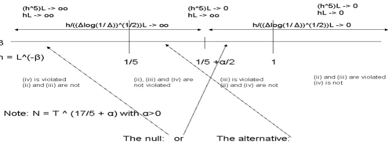
It is immediate to see that (ii) and (iii) require the bandwidth not to approach zero too fast, thus only one of the two is binding. Condition (iv) instead requires the bandwidth to approach zero fast enough. It is important to rule out the possibility of a bandwidth which is too large to satisfy (iv) and too small to satisfy the most stringent between (ii) and (iii). To this extent, we only ought to provide primitive conditions onN andT. If (iv) is violated, thenhdrN;T goes to zero not faster thanLX(T; a) 1=5: This ensures that (ii) is satis…ed, but does not ensure that (iii) is satis…ed. For (iii) to be satis…ed when (iv) is not, we needLX(T; a)6=5 1N;T=2 log(1= N;T)!0:BecauseLX(T; a)can grow at most at rateT; a su¢cient condition is thereforeN=T17=5 ! 1.
ProvidedN=T17=5 ! 1;there are three possibilities (see Figure 1). First, we have chosen the right
bandwidth and thusbhdr
N;T satis…es (ii), (iii), and (iv). Second, we have chosen too large a bandwidth, so that (ii) and (iii) hold, but (iv) is violated. Third, we have chosen too small a bandwidth, so that either (ii) or (iii) is violated (or both) but (iv) holds. Hence, at most one set of conditions can be violated, namely either (iv) or the most stringent between (ii) and (iii). To this extent, we consider the following hypotheses:
H0dr : bhdr;N;T5LbX(T; a)a:s:! 1or max
8 < :
1 bhdr
N;TLbX(T; a) ;
b
LX(T; a) N;T1=2 log1=2(1= N;T)
bhdr N;T
9 = ;
a:s:
! 1,
HAdr : bhdr;N;T5LbX(T; a)a:s:! 0 and max
8 < :
1 bhdr
N;TLbX(T; a) ;
b
LX(T; a) N;T1=2 log1=2(1= N;T)
bhdrN;T
9 = ;
a:s:
! 0.
The null is that eitherbhdr;N;T5LbX(T; a)a:s:! 1;(iv) is violated, ormin bhdrN;TLbX(T; a);
b
hdr N;T
b
LX(T;a) 1=2N;Tlog1=2(1= N;T)
a:s:
! 0;(ii)^(iii) is violated. Since it is impossible that neither (ii)^(iii) nor (iv) hold, the alternative is that both (ii)^(iii) and (iv) hold. Thus, if we reject the null, we can rely onbhdrN;T for drift estimation.
If, instead, we fail to reject the null, depending on which condition we fail to reject, we know whether we have chosen a bandwidth which is too small or one which is too large. Suppose that the selected bandwidth is too large, we proceed sequentially by choosing a smaller bandwidth until we reject the null. Because at all steps the probability of rejecting the null when it is wrong is asymptotically one, the procedure does not su¤er from the well-known sequential bias issue.
Importantly, rejection of the null, as stated above, does not rule out the possibility thatbhdr;N;T5LbX(T; a) = Op(1) (if bhdrN;T / LbX(T; a) 1=5) or min bhdrN;TLbX(T; a);
b
hdr N;T
b
LX(T;a) 1=2N;Tlog1=2(1= N;T)
= Op(1) (if bhdrN;T /
b
Figure 1: Graphical representation of the drift bandwidth test
hypotheses as follows:
H00;dr : Z
A
bhdr;N;T(5 ")LbX(T; a)daa:s:! 1
or max 8 < :
1 R
Abh
dr;(1+")
N;T LbX(T; a)da ;
Z
A b
LX(T; a) N;T1=2 log1=2(1= N;T)
b
hdr;N;T(1+") da
9 = ;
a:s:
! 1
forA D;and" >0arbitrarily small, versus
HA0;dr : negation ofH00;dr.
The role of the integral over A, and of" >0, is to ensure that rejection of the null implies
min RAbhdrN;TLbX(T; a)da;
b
hdr N;T
R
ALbX(T;a)
1=2
N;Tlog(1= N;T)da
a:s:
! 1 and RAbhdr;N;T5LbX(T; a)daa:s:! 0. However, of course, if we choose an"which is not small enough, we run the risk of not having a bandwidth sequence for whichH00;dr is rejected. Hereafter, we consider the following statistic:
VR;N;T = min
n e
V1;R;N;T; min
n e
V2;R;N;T;Ve3;R;N;T
oo
; where fori= 1;2;3
e
Vi;R;N;T =
Z
U
Vi;R;N;T2 (u) (u)du,
withU = [u; u]being a compact set,RU (u)du= 1; (u) 0 for all u2U;and
Vi;R;N;T(u) =
2 p
R R
X
j=1
1fvi;j;N;T ug
and
v1;j;N;T = exp
Z
A
bhdr;N;T(5 ")LbX(T; a)da
1=2
1;j;
v2;j;N;T = exp
Z
A b
hdr;N;T(1+")LbX(T; a)da
1!!1=2
2;j;
v3;j;N;T =
0 @exp 0 @Z A b
LX(T; a) N;T1=2 log1=2(1= N;T)
b
hdr;N;T(1+") da
1 A
1 A
1=2
3;j; (9)
with( 1; 2; 3)| iidN(0; I 3R):
In what follows, let the symbolsP andd denote convergence in probability and in distribution under P ; which is the probability law governing the simulated random variables 1; 2; 3, i.e., a standard
normal, conditional on the sample. Also, letE andV ar denote the mean and variance operators under P . Furthermore, with the notation a:s: P we mean: for all samples but a set of measure 0:
Suppose thatRAbhdr;N;T(5 ")LbX(T; a)daa:s:! 1. Then, conditionally on the sample anda:s: P,v1;j;N;T diverges to 1 with probability 1=2 and to 1 with probability 1=2: Thus, as N; T ! 1; for any u 2 U; 1fv1;j;N;T ug will be distributed as a Bernoulli random variable with parameter 1=2: Fur-ther note that as N; T ! 1; for any u 2 U; 1fv1;j;N;T ug is equal to either 1 or 0; regardless of the evaluation point u; and so as N; T; R ! 1; for all u; u0 2 U; p2
R
PR
j=1 1fv1;j;N;T ug 12 and
2 p
R
PR
j=1 1fv1;j;N;T u0g 12 will converge in d distribution to the same standard normal random variable. Hence,Ve1;R;N;T !d 21 a:s: P:It is now immediate to notice that for allu2U; V12;R;N;T(u)and
e
V1;R;N;T have the same limiting distribution. The reason why we are averaging overU is simply because the …nite sample type I and type II errors may indeed depend on the particular evaluation point. As for the alternative, if RAbhdr;N;T(5 ")LbX(T; a)da a:s:! 0;(or, if
R Abh
dr;(5 ")
N;T LbX(T; a)da = Oa:s:(1)), then v1;j;N;T, asN; T ! 1, conditionally on the sample and a:s: P, will converge to a (mixed) zero mean normal random variable. Thus, p2
R
PR
j=1 1fv1;j;N;T ug 12 will diverge to in…nity at speed pR if u 6= 0 a:s: P.
Importantly, the two conditions stated in the null hypothesis are the negation of (ii), (iii), and (iv) in Proposition 1, respectively.4 As mentioned, only one of the conditions stated under the null is false, simply because the criterion cannot select a bandwidth which is too small (for the most stringent between (ii) and (iii) to be satis…ed) and, at the same time, too large (for (iv) to be satis…ed). Hence, either Ve1;R;N;T or min
n e
V2;R;N;T;Ve3;R;N;T
o
has to diverge under the null. Thus,
minnVe1;R;N;T; min
n e
V2;R;N;T;Ve3;R;N;T
oo
; conditional on the sample, and for all samples but a set of measure zero, is asymptotically 2
1 under the null and diverges under the alternative. If we reject the
null, then conditions (ii), (iii), and (iv) in Proposition 1 are satis…ed. Otherwise, if, for instance,
e
V1;R;N;T = min
n e
V1;R;N;T; min
n e
V2;R;N;T;Ve3;R;N;T
oo
3:84 and we fail to reject the null, then bhdrN;T is
4It should be noted that the rate conditions in Proposition 1 are stated in terms of L
X(T; a) instead of LbX(T; a):
However, LbX(T;a) 1N;T=2 log1=2(1= N;T)
b
hdr N;T
a:s:
! 0if, and only if, LX(T;a) N;T1=2 log1=2(1= N;T)
b
hdr N;T
a:s:
! 0;but this ensures thatLbX(T; a)
too large (and condition (iv) is violated). The same testing procedure should therefore be repeated until
e
hdrN;T = maxnh <bhN;Tdr : s.t. H00 is rejectedo:
In other words, the proposed procedure gives us a way to learn whether the conditions for consistency and (mean zero) mixed normality of the drift are satis…ed. If they are not, it gives us a way to understand which condition is not satis…ed and modify the bandwidth accordingly.
Theorem 3. Let Assumption 1 and 2 hold. Assume T; N; R! 1; N=T17=5 ! 1, and R=T !0.5
(i) UnderH00;dr;
VR;N;T !d 21 a:s: P:
(ii) UnderHA0;dr;there are ; >0 so that
P R 1+ VR;N;T > !1 a:s: P:
The test has appealing features. Speci…cation tests generally assume correct speci…cation under the null. In our case, the bandwidth is correctly speci…ed under the alternative. This is helpful in that, in theory, rejection of the null at the 5% level gives us 95% con…dence that the alternative is true and the assumed bandwidth is correctly speci…ed. Since we stop as soon as we reject the null, we do not have a sequential bias problem. Further, the critical values (those of a chi-squared random variable with 1
degree of freedom) are readily tabulated. Reliance on a classical distribution makes testing, as well as adaptation of the bandwidth in either direction should the null not be rejected, rather straightforward. It should be stressed that the limiting distribution in Theorem 3 is driven by the added randomness ; conditional on the sample and for all samples but a set of measure zero. Nonetheless, whenever we reject the null, for all samples and for95% of random draws ; the alternative is true, and so keeping the selected bandwidth is the right choice.
We now turn tohdifN;T. We will ensure thathdifN;T is small enough as to satisfy hdif;5N;T LX(T;a) N;T
a:s:
! 08a2D;
and large enough as to satisfy hdifN;T
( N;Tlog(1= N;T))1=2LX(T;a) ! 1: In order to rule out the possibility that
any bandwidth rate is either too slow to satisfy the former condition or too fast to satisfy the latter, it su¢ces to require thatN=T5 ! 1.
We can now state the hypothesis of interest as:
H0dif : Z
A b
hdif;N;T(5 ")LbX(T; a) N;T
daa:s:! 1or
Z
A b
LX(T; a) N;T1=2 log1=2(1= N;T)
bhdif;N;T(1+") da a:s:
! 1
forA D;and" >0arbitrarily small, versus
HA0 : negation of H00.
5The conditionR=T
!0is necessary only for the case in which the local time diverges at a logarithmic rate. If the local time diverges at rateTaa >0;thenRcan grow as fast as, or faster than,T:Thus, we drop the condition in the statement
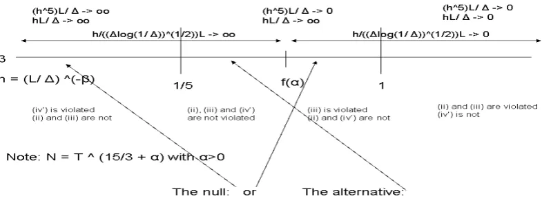
Figure 2: Graphical representation of the di¤usion bandwidth test
Remark 1. We note that, contrary to the drift case, we are not writing the second condition in the null
hypothesis as
max 8 < :
N;T
R Abh
dif;(1+")
N;T LbX(T; a)da ;
Z
A b
LX(T; a) N;T1=2 log1=2(1= N;T)
b
hdif;N;T(1+") da
9 = ;
a:s:
! 1: (10)
In fact, in spite of the fact that bhdifN;TLbX(T;a)
N;T is the rate of convergence of the di¤usion estimator, we do
not need to explicitly require its divergence (in Proposition 1, for example). If (iii) is satis…ed for the di¤usion estimator, then bhdifN;TLbX(T;a)
N;T is guaranteed to diverge. In other words, the maximum in Eq. (10)
is always the second term and the …rst term can be dropped. The graphical manifestation of this result is the fact that, in Figure 2,f(a)< 12:In the case of the drift, the maximum may vary depending on (see Figure 1). For instance, if is larger than 8
5, then the maximum condition is always R 1
AbhdrN;TLbX(T;a)da
since 1
5 + 2 >1.
Consider the following statistic:
V DR;N;T = min
n g
V D1;R;N;T; V Dg2;R;N;T
o
; where fori= 1;2
g
V Di;R;N;T =
Z
U
V D2i;R;N;T(u) (u)du, U and de…ned as above, and
V Di;R;N;T(u) = p2 R
R
X
j=1
1fvdi;j;N;T ug 1
with
vd1;j;N;T =
0 @exp
Z
A 0 @bh
dif;(5 ")
N;T LbX(T; a) N;T
da
1 A
1 A
1=2
1;j;
vd2;j;N;T =
0 @exp
0 @Z
A b
LX(T; a) N;T1=2 log1=2(1= N;T)
b
hdif;N;T(1+") da
1 A
1 A
1=2
2;j;
with( 1; 2)| iidN(0; I 2R):
Theorem 4. Let Assumption 1 and 2 hold. Assume T; N; R! 1 and N=T5! 1. (i) UnderH0dif;
V DR;N;T !d 21 a:s: P:
(ii) UnderHAdif;there are ; >0 such that
P R 1+ V DR;N;T > !1a:s: P:
Remark 2 (The local polynomial and local linear case). Our discussion has focused on classical
Nadaraya-Watson kernel estimates. We will continue to do so throughout this paper. This said, the methods readily apply to alternative kernel estimators when appropriately modi…ed, if needed. For example, they apply (unchanged) to the local linear estimates studied by Fan and Zhang (2003) and Moloche (2004).
3
Jump-di¤usion processes
We now study the problem of bandwidth selection in the context of processes with discontinuous sample paths. Consider the class of jump-di¤usion models
dXt= (Xt)dt+ (Xt)dWt+ dJt;
wherefJt:t= 1; :::; Tg is a Poisson jump process with in…nitesimal intensity (Xt)dt and jump size c. Letc=c(Xt; y), where y is a random variable with stationary distribution fy(:).
We begin by assuming existence of consistent estimates of (:) and (:) in the presence of jumps (bN;T(:) and b2N;T(:)). Later we show how these estimates can be de…ned. Write, as earlier,
b"i N;T =
Xi N;T X(i 1) N;T bN;T(X(i 1) N;T) N;T
bN;T(X(i 1) N;T)
p
N;T
b
"i N;T =
Xi N;T X(i 1) N;T bN;T(X(i 1) N;T) N;T
bN;T(X(i 1) N;T)
p
N;T
= Xi N;T X(i 1) N;T (X(i 1) N;T) N;T
(X(i 1) N;T) +op(1)
p
N;T
+op(1)
(X(i 1) N;T) Wi N;T W(i 1) N;T
(X(i 1) N;T) +op(1) p N;T
+ Ji N;T J(i 1) N;T
(X(i 1) N;T) +op(1) p N;T
+op(1)
N(0;1) + Ji N;T J(i 1) N;T
(X(i 1) N;T)
p
N;T
+op(1): (11)
If there is a jump at i N;T; Ji N;T J(i 1) N;T =Op(1). However, over a …nite time span T ; there
will only be a …nite number of times in which 1fb"i N;T xg is 1 instead of 0 or viceversa, because of
jumps. Thus,
1
N 1
N
X
i=2
1fb"i N;T xg=
1
N 1
N
X
i=2
1fb"ci N;T xg+Op(1)
N ;
whereb"ci N;T is the residual that would prevail in the continuous case. Hence, the same criterion as in Subsection 2.2 can be applied to the case with jumps.
It still remains to establish conditions under which we have consistent estimates of the in…nitesimal moments in the presence of jumps. Hereafter, we rely on the following assumption:
Assumption 3.
(i) (:); (:); c(:; y);and (:)are time-homogeneous,B-measurable functions on D= (l; u)with 1
l < u 1; where B is the -…eld generated by Borel sets on D. All functions are at least twice continuously di¤erentiable. They satisfy local Lipschitz and growth conditions. Thus, for every compact subset J of the range of the process, there exist constants CJ
4; C5J, and C6J so that, for all
x and z in J,
j (x) (z)j+j (x) (z)j+ (x) Z
Y j
c(x; y) c(z; y)j (dy) C4Jjx zj; and
j (x)j+j (x)j+ (x) Z
Y j
c(x; y))j (dy) C5Jf1 +jxjg; and for >2;
(x) Z
Y j
c(x; y))j (dy) C6Jf1 +jxj g;
(iii) (:); (:); c(:; y);and (:) are such that the solution is recurrent.
In what follows, we consider two alternative scenarios. First, we establish the validity of our band-width selection procedure for all in…nitesimal moments under parametric assumptions on the jump component. Second, without making parametric assumptions on the jump component, we discuss band-width selection for the purpose of consistent (and asymptotically normal) estimation of the system’s drift and in…nitesimal variance. In the former case, we incur the risk of incorrectly specifying the jump distribution but completely identify the system’s dynamics. The procedure is, in spirit, semiparametric. In the latter case, we are agnostic about the jump distribution, but can only identify the process’ drift (possibly inclusive of the …rst conditional jump moment) and the process’ in…nitesimal volatility, while remaining fully nonparametric. If interest is on the full system’s dynamics, one should employ the proce-dure in Subsection 3.1. If interest is solely on the volatility of the continuous component of the process, then the methods in Subsection 3.2 are arguably preferable. As we will show, in fact, the di¤usion’s kernel estimator converges at a faster rate in this second case.
3.1 Consistent estimation of all in…nitesimal moments
In order to separate the moments of the continuous component from those of the jump component, we ought to properly correct the kernel estimators considered in the previous section. Following Bandi and Nguyen (2003) and Johannes (2004), de…ne
bN;T(a) =
1
N;T
PN 1
j=1 K
Xj N;T a
hn;T;1 X(j+1) N;T Xj N;T
PN
j=1K
Xj N;T a
hN;T;1
bhn;T(Xt)Eby;hn;T(c(Xt; y)) (12)
and
b2N;T(a) =
1
N;T
PN 1
j=1 K
Xj N;T a
hn;T;2 X(j+1) N;T Xj N;T
2
PN
j=1K
Xj N;T a
hN;T;2
bhn;T(Xt)Eby;hn;T c(Xt; y)2 : (13)
Since the intensity estimatorb(:);as well as the jump size moment estimator, Eby c(:; y)j withj= 1;2 depend, in general, on higher-order in…nitesimal moment estimates, we make explicit their dependence on a (vector-)bandwidthhn;T and write bhn;T(:) andEby;hn;T c(:; y)2 , as above.
We are now more speci…c. Identi…cation of (:) and the moments of the jumps may hinge on
b
Ey;hn;T c(Xt; y)2 = b2y N;T =
1
N N
X
j=1 c
MN;T;h6 6(Xj n;T)
5Mc4
N;T;h4(Xj n;T)
;
bhn;T(a) =
c
M4
N;T;h4(a)
3 b4y N;T ;
with
c
MN;T;hj
k(a) =
1
N;T
PN 1
j=1 K
Xj N;T a
hn;T;k X(j+1) N;T Xj N;T
j
PN
j=1K
Xj N;T a
hN;T;k
j= 1; :::
Since the mean of the jump size is zero, Eq. (12) and Eq. (13) become, in this case:
bN;T(a) = McN;T;h1 1(a); (14)
b2N;T(a) = McN;T;h2 2(a)
c
MN;T;h4 4(a)
3 1
N
PN
i=1 c
M6
N;T;h6(Xi n;T)
5Mc4
N;T;h4(Xi n;T)
2 0
@1
N N
X
i=1 c
MN;T;h6 6(Xi n;T)
5Mc4
N;T;h4(Xi n;T)
1
A; (15)
with hn;T = (h1; h2; h4; h6). In other words, optimization of the criterion in Subsection 2.2 will now depend on four bandwidths whose properties are laid out below.
Proposition 2 (Bandi and Nguyen, 2003): Let Assumption 3 hold.
(i) Let N;T =T =N withT …xed. If limN!1hN;T1 N;Tlog 1
N;T
1=2
!0, then
b
LX(T ; a) LX(T ; a) =oa:s:(1);
whereLbX(T ; a) = hN;T
N;T
PN
j=1K
Xj
N;T a
hN;T :
The in…nitesimal moments
If (ii) hN;T;kLX(T; a)a:s:! 1 and (iii) LhXN;T;k(T;a) N;Tlog N;T1
1=2 a:s:
! 0;then:
c
MN;T;hk k(a) Mk(a) =oa:s:(1): If, in addition, (iv) hdr;N;T;k5 LX(T; a)a:s:! 0;then:
q
hN;T;kLbX(T; a) McN;T;hk k(a) M
k(a) )N 0;K
2M2k(a) :
From the proposition above, we note that all moments estimators converge to their limit at the same rate,
q
for all moments. This is in sharp contrast with the continuous semimartingale case in which the drift estimator converges at a slower rate than the in…nitesimal variance estimator. In the continuous case, in fact, one ought to use di¤erent bandwidth rates, since, from the conditions in Proposition 1, we require hdr
N;TLX(T; a)a:s:! 1 (for the drift bandwidth) andhN;Tdif LX(T; a)a:s:! 0 (for the di¤usion bandwidth).6 LetbN;T;h(a) and b2N;T;h(a)be de…ned as in Eq. (14) and Eq. (15) withh1=h2 =h4 =h6=h: We
can now selecthin such a way as to minimizesupxjFN;T;h(x) (x)j;whereFN;T;h(x) is the empirical distribution ofb"(as de…ned in (11)) evaluated atx:Given the nature of the bandwidth requirements from Proposition 2, the second-step procedure can be carried out as in the continuous drift case. Similarly, the asymptotic behavior of the second-step procedure is as established in Theorem 3.7
Needless to say, misspeci…cation of the parametric distribution of the jump component will, in general, result in failure of the statement in Theorem 2 since, in this case, there might not exist a bandwidth for which supxjFN;T;h(x) (x)j=op(1): We now turn to a procedure which does not impose parametric assumptions on the process’ discontinuities at the cost of solely identifying the moments of the process’ continuous component.
3.2 Consistent estimation of the drift and in…nitesimal variance
Should we be unwilling to make parametric assumptions on the distribution of the jump component, we may still consistently estimate the in…nitesimal variance term. The only maintained assumption about the jump component in this subsection is thatJt is a process of …nite activity. De…ne b2J;N;T(a)as:
b2J;N;T(a) =
p
2=p
N;T
PN p
j=1 K
Xj N;T a
hdifN;T
p
i=1 X(j+i) N;T X(j+i 1) N;T 2 p
PN
j=1K
Xj N;T a
hdifN;T
; (16)
where k= E jZjk ;withZ denoting a standard normal random variable, and2< p < p <1: Corradi and Distaso (2008) have studied the properties of this class of estimators for the case N;T =
T
N withT …nite. They have shown that, under mild conditions,b
2
J;N;T(a)identi…es 2(a)consistently in
the presence of …nite activity jumps. Since we are also dealing with …nite activity jumps, with probability one we can have at most a …nite number of jumps over a …nite time span. As the time span increases inde…nitely, the number of jumps increases roughly at the same rate. Providedp >2;asymptotic mixed normality follows under the same rate conditions as in the continuous semimartingale case. Theorem 5 states the relevant result.
6Consider conditions (iii) and (iv’) in Proposition 1. From (iv’), we notice that
N;T has to vanish at a slower rate
thanhdif;5N;T LX(T; a):Set N;T =O hdif;5N;T LX(T; a) with >0arbitrarily small. Now, plugging this condition into (iii)
and ignoring the logarithm, we obtain
LX(T; a)
hdifN;T
q
hdif;5N;T "LX(T; a) =L 3=2
X (T; a)hdif;3=2N;T "=2 a:s:
! 0;
which implieshdifN;TLX(T; a)a:s:! 0but, of course, this is in contraddiction with (ii) in the drift case (see Proposition 1).
7Simulations suggest that it is sometimes very bene…cial to select a smaller bandwidth for the in…nitesimal second
moment than for the …rst and higher-order moments (see, e.g., Bandi and Renò, 2008). One may therefore seth1=h4=h6
Theorem 5. Let Assumption 3 hold and let p > 2. If (i) LX(T;a)
hdifN;T N;Tlog
1
N;T
1=2 a:s:
! 0 and (ii) hdif;5N;T LX(T;a)
N;T
a:s:
! 0, then v u u
thdifN;TLbX(T; a)
N;T b
2
J;N;T(a) 2(a) )N 0; pK2 4(a) ;
where
p = p
4=p (2p 1)
2p
2=p+ 2 p 1 4=p 22=p+
p 2
4=p 42=p+:::+
p (p 1) 4=p
2(p 1) 2=p
2p
2=p
:
Let
b
"i N;T =
Xi N;T X(i 1) N;T bN;T(X(i 1) N;T) N;T
bJ;N;T(X(i 1) N;T)
p
N;T
;
wherebN;T is de…ned as in (14) andb2J;N;T(a)is as in (16) above withp >2:We may now selecthN;T =
(hdrN;T; hdifN;T) so as to minimize supxjFN;T;h(x) (x)j;whereFN;T;h(x) is the empirical distribution of
b". Subsequently, we can verify the rate conditions as in the continuous semimartingale drift and di¤usion case. In other words, Theorems 3 and 4 apply.
Of course, if the jump size does not have mean zero, the procedure only identi…es the sum of the drift component and the compensator (see, e.g., Eq. 12) while remaining consistent for the di¤usive volatility. Should this be the case, then one has to resort to parametric assumptions, as in the previous subsection, to identify the continuous drift component, if needed.
4
Di¤usions observed with error (or microstructure noise)
We now assume that the processXt is contaminated by measurement error and write observations from the observable processYt as
Yi N;T =Xi N;T + i N;T; (17)
whereaN;T1=2 i N;T is an i.i.d. sequence with mean zero, variance1, and such that E
k
i N;T =O a
k=2
N;T (k 2) for aN;T !0 asN; T ! 1:
We provide estimates of the …rst two in…nitesimal moments which are robust to this type of mea-surement error. In this context, we establish conditions for consistency and asymptotic normality. We then turn to the issue of automatic bandwidth choice. Write
bN;l;T(a) =
PB
b=1 Pl 1
j=1K
Y((j 1)B+b) N;T a
hdr N;l;T
1
l;T Y(jB+b) N;T Y((j 1)B+b) N;T
PB
b=1 Pl 1
j=1K
Y((j 1)B+b) N;T a
hdr N;l;T
whereBl=N and l;T =T =l. As for the di¤usion:g
b2N;l;T(a) =
PB
b=1 Pl 1
j=1K
Y((j 1)B+b) N;T a
hdifN;l;T
1
l;T Y(jB+b) N;T Y((j 1)B+b) N;T
2
PB
b=1 Pl 1
j=1K
Y((j 1)B+b) N;T a
hdifN;l;T
1
l;TRVT;N N;T;
(19) whereRVT;N N;T = N;TPNj=1 Yj N;T Y(j 1) N;T
2
:In the case of a …xed time span, the estimator in Eq. (19) has been studied by Corradi and Distaso (2008). Here, we also consider estimation of the …rst in…nitesimal moment as in Eq. (18). In both cases, letting the time span increase without bound (which is, as always, necessary in the drift case for consistency) raises additional technical issues which ought to be dealt with.
Remark 3 (market microstructure). When Yi N;T is an observable logarithmic price process (i.e.,
a transaction price or a mid-quote, for example),Xi N;T generally denotes the underlying, unobservable
equilibrium price and"i N;T de…nes market microstructure noise. If econometric interest is placed on the
drift and di¤usion function of the equilibrium price process, as is generally the case, thenbN;l;T(a) and
b2N;l;T(a) will provide consistent and asymptotically normal estimates of its true in…nitesimal moments (as we show below) even when contaminated price observationsYi N;T are employed.
Remark 4. We note that the form ofbN;l;T(a)and b2N;l;T(a)requires the use of an appropriately-chosen lower frequencyl. In agreement with the two-scale estimator of Zhang, Mykland, and Aït-Sahalia (2005), ZMA henceforth, the di¤usion case also requires a bias-correction term based on the higher frequency N (see, also, Aït-Sahalia, Mykland, and Zhang, 2009).
Theorem 6
The in…nitesimal …rst moment
Let Assumption 1 hold and let be de…ned as in Eq. (17). Also assume that l = O(BT): If (i) hdrN;l;TLX(T; a) a:s:! 1; (ii) LhXdr(T;a)
N;l;T l;T
log 1
l;T
1=2 a:s:
! 0; (iii) hdr;N;l;T5 LX(T; a) a:s:! 0, and (iv) N1=ka1=2
N;T
p
LX(T;a)
q
hdr N;l;T
a:s:
! 0;then
r
hdrN;l;TLbX(T; a) bN;l;T(a) (a) )N 0;
2 3K2
2(a) :
The in…nitesimal second moment
Let Assumption 1 hold and let be de…ned as in Eq. (17). Also assume that l = O(BT): If (i)
LX(T;a)
hdifN;l;T l;Tlog
1
l;T
1=2 a:s:
! 0;(ii) hdif;5N;l;TLX(T;a) l;T
a:s:
! 0;(iii) a2N;Tl 2 l;T !
0;and (iv) N1=ka
1=2 N;Tl1=2
r
hdifN;l;TLX(T;a) T
hdifN;l;T
a:s:
!
0;then v
u u
thdifN;l;TLbX(T; a)
l;T b
2
Both in the drift and in the di¤usion case, the averaging over sub-grids reduces the constant of propor-tionality in the estimators’ asymptotic variance (from1to 2
3 in the drift case, from2to1in the di¤usion
case). The rates of convergence are also a¤ected. In the di¤usion case, since N;T
l;T ! 0, the rate is
slower. In the drift case, the new bandwidth condition (ii) requires larger bandwidth choices and thus, compatibly with condition (iii), the actual rate may be faster. Since N =Bl; by choosing a smaller l, and hence a larger B, we may allow for a larger variance of the error term. This choice will in general not come at a price (in terms of convergence rate) as far as the drift is concerned, but could come at a price in the case of di¤usion estimation if h
dif N;l1;T
l1;T =o
hdifN;l
2;T
l2;T withl1 < l2.
Turning to bandwidth selection, we note that our local Gaussian criterion ought to be re-adjusted in this new framework. We …rst propose a heuristic argument to provide intuition. Let
b
ui N;T =
Yi N;T Y(i 1) N;T bN;l;T(Y(i 1) N;T) N;T
bN;l;T(Y(i 1) N;T)
p
N;T
= Yi N;T Y(i 1) N;T (Y(i 1) N;T) N;T
(Y(i 1) N;T) +op(1) p N;T
+op(1)
= Xi N;T X(i 1) N;T (X(i 1) N;T) N;T + i N;T (i 1) N;T
0(X
(i 1) N;T) (i 1) N;T N;T
(X(i 1) N;T) + 0(X(i 1) N;T) (i 1) N;T +op(1)
p
N;T
+op(1)
= ui N;T +op(1);
where X(i 1) N;T 2 X(i 1) N;T; Y(i 1) N;T :In spite of the consistency of the drift and in…nitesimal variance estimator, ui N;T is in general non-Gaussian since the presence of measurement error a¤ects
Yi N;T Y(i 1) N;T and, of course, the evaluation point.
A natural solution to this issue is to use di¤erent frequencies for in…nitesimal moment estimation and for bandwidth selection. For the latter, one may use a (lower) frequency at which the contamination error is expected to have little or no e¤ect, say H;T; with H=N ! 0: Provided aN;T = o( H;T); we de…ne
b
ui H;T =
Yi H;T Y(i 1) H;T bN;l;T(Y(i 1) H;T) H;T
bN;l;T(Y(i 1) H;T)
p
H;T
= Xi H;T X(i 1) H;T (X(i 1) H;T) H;T
(X(i 1) H;T) +op(1) p H;T
+op(1)
= ui H;T +op(1):
It is now clear thatui H;T is approximately Gaussian. The criterion de…ned in Section 2.2 is therefore
Remark 5. In the case of high-frequency logarithmic asset prices and market microstructure noise, an appropriate frequency may be chosen in a data-driven manner, either by looking at signature plots (Andersen, Bollerslev, Diebold, and Labys 2000) or via the statistics suggested by Awartani, Corradi, and Distaso (2009).
In the second stage one needs to verify whether the bandwidths selected by the procedure in Theorem 1, saybhdr
N;l;T andbh dif
N;l;T, satisfy all of the rate conditions in Theorem 6. We begin with the drift. Notice thatN; T and the size of the measurement erroraN;T are given. WhileaN;T is unknown in general, it may be estimated by using(RVT;N N;T)=2 as de…ned in Eq. (19). Given N, we …x l and B, using the fact thatN =lB: If we choosel=O aN;T1 T ;it is immediate to see that (ii) implies (iv). Summarizing, if T17=5=l!0and l=O a 1
N;TT ;there is a bandwidth satisfying (i)-(iv) and we can proceed along the lines of Theorem 2 by testing the hypothesis:
H0dr : Z
A
bhdr;N;l;T5 "LbX(T; a)daa:s:! 1
or max 8 < :
1 R
Abh
dr;(1+")
N;l;T LbX(T; a)da ;
Z
A b
LX(T; a) l;T1=2log1=2(1= l;T)
b
hdr;N;l;T(1+") da
9 = ;
a:s:
! 1
forA D;and " >0 arbitrarily small, versus its alternative.
We now turn to the variance estimator. If we set l = O aN;T2=3+"T2=3 ; (iii) is always satis…ed.
Further, ifT5=l!0;there is a bandwidth satisfying (i) and (ii). We now test the following hypothesis:
H0dif : Z
A b
hdif;N;l;T5 "LbX(T; a) l;T
daa:s:! 1 or
max 8 > > < > > : Z
A
N1=ka1N;T=2l1=2
r
hdifN;l;TLbX(T;a)
T
hdif;N;l;T(1+") da;
Z
A b
LX(T; a) l;T1=2log1=2(1= l;T)
b
hdif;N;l;T(1+") da;
9 > > = > > ;
a:s:
! 1
forA D;and " >0 arbitrarily small, versus its alternative.
5
Stochastic volatility
Consider now the model
dXt = Xt dt+vtdWtX df(vt2) = (v2t)dt+ (v2t)dWt;
where WtX :t= 1; :::; T and fWt :t= 1; :::; Tg are potentially correlated Brownian motions. The functionf(x)may be equal tolog(x)as in Jaquier, Polson, and Rossi (1994) orxas in Eraker, Johannes, and Polson (2003), for instance. Our interest is in (v2t)and 2(v2
Volatility is latent. However, it may be …ltered from pricesXtsampled at high frequency as suggested by Kristensen (2008) and Bandi and Renò (2008). To this extent, assume, as earlier, availability ofN equidistant price observations with N;T = T =N denoting the time distance between successive data points and T denoting the time span. We again observe the price skeleton X N;T; X2 N;T; :::; XT N;T.
These price observations may be employed to (1) …lter spot volatility (or spot variance) nonparametrically for the purpose of (2) identifying (:)and 2(:). Using preliminary spot variance estimatesbv2
t, the latter may be done by virtue of the functional estimators in Eq. (1) and (2) (Bandi and Renò, 2008, and Kanaya and Kristensen, 2008). Importantly, however, selection of the smoothing sequenceshdr andhdif now also depends on the need to eliminate the impact of the estimation error induced by the …rst-step spot variance estimates.
To present the main ideas, consider spot variance estimates obtained by virtue of the classical re-alized variance estimator (Andersen, Bollerslev, Diebold, and Labys, 2003, and Barndor¤-Nielsen and Shephard, 2002). Speci…cally, write
b
v2 =
+T N 1
N;T
X
i= T N 1 N;T
T N X
(i+1) N;T Xi N;T
2
: (20)
The estimator averages 2T N 1
N;T squared price di¤erences in a local neighborhood of determined by the localizing factorT N.
Bandi and Renò (2008) introduce four additional conditions (with respect to those in Proposition 1 above) which the drift bandwidthhdr and the di¤usion bandwidth hdif ought to satisfy for asymptotic normality of the drift and the di¤usion function estimates to hold. These conditions (two for each in…nitesimal moment) are su¢cient to eliminate, asymptotically, the in‡uence of the estimation error induced by bv2 (when used in place of the unobservable v2). Intuitively, the conditions imply that one
needs to use a larger discrete interval, say M;T = MT withM=N !0, than is used for estimating the preliminary spot variance estimates. In other words, one needs to use high-frequency data to identify spot variancevb2 andM lower frequency observations (onbv2) to identify the dynamics (through (:)and
2(:)). To this extent, call the relevant bandwidthshdr
M;T and h dif M;T.
In what follows, for conciseness, we will not discuss the origin and form of these four conditions. We refer the reader to Bandi and Renò (2008) and Appendix B to this paper for details. However, consistently with our stated goal, we discuss the implications of the four conditions for bandwidth choice. When dealing with this choice, the main technical issue is now that the rate of growth ofM depends onhdrM;T; which is what one needs to …nd optimally, as well as onLv(T; a) which is unknown and whose estimates depend onhdrM;T: This is an important di¤erence from the observable case in which allN observations are used. In the drift case, one may consider optimizing over both Mdr and hdr
M;T. Similarly, in the di¤usion case one might wish to optimize overMdif and hdif
M;T. We leave this issue for future work and take the following approach to the problem.
As said, it is natural for applied researchers to employN high-frequency observations to identify spot variance before usingM lower frequency data (on bv2) to evaluate the dynamics. To this extent, assume
bandwidth condition becomes:
hdrM;TLv(T; a)
0
@N
2 2 +1
T 2 2 +1
M2
1 A
| {z }
N;T;M
a:s:
! 1: (21)
where 1
2.8 As for the di¤usion:
hdifM;TLv(T; a) T;M
0
@N N
2 1+2
1 2 T
2 1+2
1 2 T
M4
1 A
| {z }
N;T;M
a:s:
! 1: (22)
In general (i.e., for empirically reasonable values of N; M; T), it is easy to see that N;T;M < 1 and N;T;M <1. Hence, Eq. (21) and Eq. (22) are more stringent conditions thathdrM;TLv(T; a) a:s:! 1and hdifM;TLv(T;a)
T;M
a:s:
! 1with probability one. This observation leads to the following tests.
If M
T17=5 ! 1andN; M; T are such that N;T;M !0andT[1 ( 1
5+c)] N;T;M ! 1(withc >0;where
T is the local time’s divergence rate), then
H0dr :bhdr;M;T5Lbv(T; a)a:s:! 1 or max
8 < :
1
N;T;MbhdrM;TLbv(T; a) ;
b
Lv(T; a) M;T1=2 log1=2(1= M;T)
b
hdr M;T
9 = ;
a:s:
! 1:
If M
T5 ! 1 and N; M; T are such that N;T;M !0 and M[1 (15+c)]T[1 (
1
5+c)]( 1) N;T;M ! 1(with c >0, whereT is the local time’s divergence rate), then
H0dif : bh
dif;5
M;TLbv(T; a) M;T
a:s:
! 1or max
8 < :
M;T
N;T;MbhdifM;TLbv(T; a) ;
b
Lv(T; a) M;T1=2 log1=2(1= M;T)
b
hdifM;T
9 = ;
a:s:
! 1:
6
Multivariate di¤usion processes
We now turn to multidimensional di¤usions. Let Xt = (X1;t; :::; Xd;t)| and consider the stochastic di¤erential equation
dXt= (Xt)dt+ (Xt)dWt;
8These conditions allow for the use of market microstructure noise-robust spot variance estimators. Bandi and Renò
(2008) propose noise-robust spot variance estimators with a rate of convergence equal to k = T N
N;T for some 1
2. As in the case of realized variance (above), these estimators may be derived from robust integrated variance
estimators (such as the two-scale estimator of Zhang, Mykland, and Aït-Sahalia, 2005, and the class of kernel estimators suggested by Barndor¤-Nielsen, Hansen, Lunde, and Shephard, 2008b) by localizing the integrated estimates in time. Their asymptotic properties (studied in Bandi and Renò, 2008) reveal that is, for instance, equal to1=10(in the case of the two-scale estimator) or1=6in the case of ‡at-top kernel estimates obtained by virtue of kernels g(:) satisfyingg0(1) = 0
where (:) and (:) are matrix functions satisfying the regularity conditions for the existence of a recurrent solution in Bandi and Moloche (2004) and fWt:t= 1; :::; Tg is a (conformable) standard Brownian vector. Let the di¤usion matrix (a) be de…ned as (a) = (a) (a)| forx= (a
1; :::; ad): Suppose we observe X N;T; X2 N;T; :::; XN N;T with N;T =
T
N:Speci…cally, assume there is a fre-quency at which synchronized observations may be observed for all processes. This is standard for estimation methods relying on low-frequency observations. In principle, however, we could allow for observations recorded at random, asynchronous times and, therefore, use high-frequency data for es-timation. This could be done, for example, by employing the refresh time approach advocated by Barndor¤-Nielsen, Hansen, Lunde and Shephard (2008a). The use of refresh times, however, would require important, additional technicalities due to their randomness, and is beyond the scope of the present paper. In particular, it would require an extension of existing asymptotic (mixed) normal results for drift and in…nitesimal variance estimators (in Proposition 3 below) to the case of random times.
We de…ne Nadaraya-Watson estimators of the drift vector and covariance matrix by writing
bN;T(a) =
1
N;T
PN 1
j=1 K
Xj N;T a hdr
N;T
X(j+1) N;T Xj N;T
PN
j=1K
Xj N;T a hdr
N;T
and
bN;T(a) = 1
N;T
PN 1
j=1 K
Xj N;T a hdif
N;T
X(j+1) N;T Xj N:T X(j+1) N;T Xj N:T
|
PN
j=1K
Xj N;T a hdif
N;T
;
where the kernel K Xj N;T x hN;T =
d i=1K
Xi;j N;T xi
hi;N;T is a product kernel and K(:) is de…ned in the
same manner as in Assumption 2. We denote byhN;T the matrix bandwidth hdr
1;N;T; :::; hdrd;N;T; h dif
1;N;T; :::; h dif d;N;T belonging to the setH R2d
+:
In the multivariate case, local time is not de…ned. However, the averaged kernel
b
LX(T; x) = d N;T i=1hi;N;T
NX1
j=1
K Xj N;T a hN;T
will still provide an estimate of the occupation density of the process (while, at the same time, inheriting its divergence rate) as discussed in Bandi and Moloche (2004). Naturally, the divergence rate of the occupation density plays a role in the characterization of the bandwidth conditions for both the drift and the di¤usion matrix.
Proposition 3(Bandi and Moloche, 2004): Let Assumption 1 and 2 in Bandi and Moloche (2004) hold.
Assume T; N ! 1 and N;T !0:Assume, for all i,hi;N;T !0 and
( n;Tlog(1= n;T))1=2= di=1hi;N;T !0: Then,
b
LX(T; a)
where the function v(1=T) is regularly-varying at in…nity with process-speci…c parameter satisfying
0 1,g is used here to denote the Mittag-Le-er random variable with the same process-speci…c parameter , and CX is a process-speci…c constant.
The drift estimator
If, for all i; hdr
i;N;T !0, di=1hdri;N;Tv(1=T)! 1;and v(1=T)
d
i=1hdri;N;T
N;Tlog
1
N;T
1=2
!0;
then
bN;T(a) (a) a:s:
! 0:
If, in addition, for allj,hdr;j;N;T5 di6=jhdri;N;Tv(1=T)!0;
r
d
i=1hdri;N;TLb dr
X(T; a) bN;T(a) (a) ) 1=2(a)N 0;Kd2Id ; whereId is ad didentity matrix.
The di¤usion estimator
If, for alli; hdifi;N;T !0;
d i=1h
dif
i;N;Tv(1=T)
N;T ! 1;and
v(1=T)
d i=1h
dif i;N;T
N;Tlog
1
N;T
1=2
!0;
then
bN;T(a) (a)a:s:! 0:
If, in addition, for allj; h
5;dif j;N;T di6=jh
dif
i;N;T v(1=T) N;T !0;
v u u t di=1h
dif i;N;TLb
dif X (T; a) N;T
vech bN;T(a) (a) )V(a)1=2N 0;Kd2Id ;
withV(a) =PD(2 (a) (a))PD|;wherePD is so that vech (a) =PDvec (a):
We now turn to the …rst step of our bandwidth selection procedure. For i= 2; :::; N;T1 T de…ne the inner product of the residual process:
b"|
i N;Tb"i N;T =
n 1
N;T X(j+1) N;T bN;T(X(j+1) N;T) N;T
|
bN;T(X(j+1) N;T) 1 X(j+1) N;T bN;T(X(j+1) N;T) N;T
o
; where X(j+1) N;T =X(j+1) N;T X(j+1) N;T:Now write:
b
hN;T = arg min
h
1
N 1usup2D+
N
X
i=2
1nb"|
i N;Tb"i N;T u
o
and
h
N;T =h2H R+2d: sup
x Fh
N(x) (x)
p
!
N;T!1; N;T!0
0;
where (u) = Pr 2d u , i.e., the cumulative distribution function of a Chi-squared random variable withddegrees of freedoms. Note that
b"i N;T
= "i N;T + bN;T(X(j+1) N;T)
1=2 (X
(j+1) N;T)
1=2 1=2
N;T X(j+1) N;T
+ (X(j+1) N;T)
1=2 b
N;T(X(j+1) N;T) (X(j+1) N;T
p
N;T
+ bN;T(X(j+1) N;T)
1=2 (X
(j+1) N;T)
1=2 b
N;T(X(j+1) N;T) (X(j+1) N;T
p
N;T; where "i N;T = (X(j+1) N;T)
1=2 1=2
N;T X(j+1) N;T (X(j+1) N;T)
p
N;T ;and so "|i N;T"i N;T
is i.i.d. 2
d: Hence, as N; T ! 1 and N;T ! 0; by the same arguments as in Theorem 1 and 2,
b
hN;T h
N;T p
!0 if, and only if,
sup
a2Dd bN;T
a;hbdr
N;T (a) =op
1 p N;T ! ; (23) and sup
a2Dd
vech bN;T a;hbdifN;T (a) =op(1): (24)
In the second step, we need to check whetherhbdr
N;T is small enough as to satisfy (i)maxjh5j;N;T;dr di6=jhdri;N;TLb
dr X(T; a)
a:s:
! 08a2Ddand large enough as to satisfy max
(
(ii) 1
d
i=1hdri;N;TbL dr X(T;a)
; (iii) ( N;Tlog(1= N;T))1=2bL dr X(T;a) d
i=1hdri;N;T
)
a:s:
! 1 8a 2 Dd: Similarly, we need to
check whether hdif
N;T is small enough as to satisfy
maxjh5;difj;N;T di6=jh dif i;N;TbL
dr X(T;a) N;T
a:s:
! 0 8a 2 Dd and large
enough as to satisfy di=1h dif i;N;T
( N;Tlog(1= N;T))1=2Lb dif X (T;a)
a:s:
! 1:Let us begin with the drift estimator. Without any restriction on the relative (almost-sure) order of the various bandwidths, we cannot ensure that there is a vectorhN;T so that whenever (i) is violated, (ii)-(iii) cannot be violated. This may happen when maxjh5j;N;T;dr di6=jhdri;N;TLb
dr X(T; a)
a:s:
! 1 butminjh5j;N;T;dr di6=jhdri;N;TLb dr X(T; a)
a:s:
! 0: Broadly speaking, (ii)-(iii) only depend on the product on the bandwidths, while (i) depends both on the product and on the individual bandwidths. Therefore, in order to ensure the existence of bandwidths satisfying all conditions, we need to impose some restrictions on the degree of "heterogeneity" of their almost-sure order. We require that, for all j; hdrj;N;T = Oa:s: di6=jhdri;N;T
1=(d 1)
; so that the bandwidths can di¤er from each other but are of the same almost-sure order. Given that, whenever (i) is violated,
d
i6=jhdri;N;T approaches zero almost surely at a rate equal or slower than Lb dr X(T; a)
d 1
d+4;and d
i=1hdri;N;T cannot approach zero at a rate faster than LbdrX(T; a) d+4d ; it is immediate to see that (ii) is trivially