Spatial Air Quality Prediction Using Gaussian Process

2018 International Conference on Computer, Communications and Mechatronics Engineering (CCME 2018) ISBN: 978-1-60595-611-4

Spatial Air Quality Prediction Using Gaussian Process

Wei-wei GU

, Chun-xiu XI

, Rui LIU

, Tao XIE

and Xiao-hong XU

1_{China Science Map Universe Technology Co., Ltd., China} 2

University of Windsor Canada

*

Corresponding author

Keywords: PM2.5, Non-linear regression, Gaussian process, Real deployment dataset.

Abstract. The exponential development of economy has evoked the problem of environment, particularly the PM2.5, which is extremely detrimental to people’s health and has gained high attention from the public. Under contemporary circumstance, current software that report the level of PM2.5 is limited by the city level. Thus, with the intension to help people aware the exact air quality of surrounding areas, we installed 280 fine designed devices to these places and presented a Gaussian Process based inference model to estimate the value at any place. Based on the real data and compared to related methods, the experimental results of proposed method prove the effectiveness of it.

Introduction

The air pollution is an exceed problem even at the global range, such as Beijing and New Delhi of the developing country. What has gained the most attention of the public is the particular matter (PM) with diameters less than 2.5 micron, well known as PM2.5. PM2.5 can be easily absorbed by lungs and hardly to be metabolized, as a result, multiple kinds of diseases is stimulated by its accumulation, such as blood disease or lung cancer. The increasing cases of disease has forced people to care about the air quality so that they will find a way to prevent both themselves and their children from it.

Depend on this condition, better ways to monitor the air quality are the importance of people’s life. Unfortunately, existing web or smart phone applications only report publicly-available air quality data at the city or district level, but fail to calculate the precise air quality taken by people, which is relatively significant to people’s life and health. In fact, there is probably a significant difference between the values of PM2.5 concentration at different locations of the district level, which has been attested by the real data as shown in experiment section. Consequently, it is highlighted to find a fine-grained air quality monitoring system for this problem.

During the past years, two major classical ways are applied to estimate the air quality of any location. One is classical dispersion models, such as Gaussian Plume models, Operational Street Canyon models, and Computational Fluid Dynamics. These models are normally a function of meteorology, street geometry, receptor locations, traffic volumes, and emission factors (e.g., g/km per single vehicle), based on numerous empirical assumptions that might not be applicable to all urban environments and parameters which are also difficult to obtain precisely. Another one is interpolation using reports from nearby air quality monitor stations. This method is usually adopted by public websites releasing the air quality index (AQI).

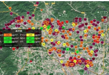
Figure 1. The sensor deployment in Changping, Beijing.

To overwhelm the drawbacks of existing methods shown above, we designed a PM2.5 monitoring system which is composing of a sensor network and an inference model. The sensor network that is deployed among where are monitored to provide the values of PM2.5. Thus, our situation is basically distinctive from ``U-Air'', since our PM2.5 monitoring devices are designed and deployed at a much higher density (280 monitor stations over a 20km by 20km urban area, as shown in Figure1), which provides relevantly more sufficient data for air quality estimation. Albeit the flaws of our cheap PM2.5 devices limit the capacity of precision, which is not as accurate as the measurement precision of expensive public monitor stations, they are precise enough for the air quality estimation after calibration. Hence, we simply regard their readings as ground truth, and we mainly focus on the development of an effective model to estimate the value of PM2.5 at any place using the acquired data at such a relatively higher deployment density.

The paper is organized as follows: in system section, a description of the system is given. The inference model based on Gaussian Process is detailed in model section. The experiment setup and evaluation results are given in Section experiment, and the conclusions are drawn in conclusion section.

Models

In this section, we detail the Gaussian Process based inference module that estimates the value of PM2.5 using the data from the monitoring network. First, we model the inference module as a regression after some necessary definitions. Then the problem is solved as a Gaussian Process regression and the details are presented.

Problem Definiton and Regression Model

Using x_i to denote the coordinates of the i-th monitoring station and y_i the value of PM2.5 at this

place, the objective of the inference module is to inference the value of PM2.5 y at any place given the data from all monitoring stations _{{( ,y), 1, , }i n} 2

i i

 x    and the coordinate of the place to be estimate

X. This is a typical regression problem which is usually formulated as

, 2

( ) ~ (0, )

y f e e

i  xi  i i  ₍₁₎

where _ei is the noise term and the objective is to learn a proper f from which can predict a proper y for any given x.

Gaussian Process Regression

A Gaussian process is a collection of random variables, any finite number of which have consistent joint Gaussian distributions. In Gaussian process regression problems, latent function f behaves

following a Gaussian distribution (Normal distribution) when conditioning on x

1 2 1 2

( ,f f ,,f_n| , ,, _n) (0,K)

P x x x

(2) Where f_if(x_i) is latent function and K is a covariance matrix with entries given by the covariance

function, K_ijk(x x_i, _j). k(x x_{1 2}, ) can be any valid kernel function satisfying Mercer's condition.

In inference, the training and test latent values is denoted asf[f_{1 2},f , ,f_n], f_*[f_{*1 *2},f , ,f_*n]

separately, we combine the prior with the likelihood function via Bayes rule obtaining the posterior distribution: * * ( , ) ( | ) ( , | ) ( )

 P f f P y f

P f f y

P y ₍₃₎

The desired posterior predictive distribution can be produced by marginalizing out the training set latent variables f in equation:

* *

1

( | ) ( , ) ( | )d ( )



_

P f y P f f P y f f

P y ₍₄₎

Since the prior and the likelihood function are mutually independent and both follow Gaussian distribution as , *, ,* *,* * 2 ~ , , | ~ ( , ) K K K K I        _{ }   _{ }     

f f f

f

f

0 f

y f f ₍₅₎

Where _2 _{is the noise variance and I is the identity matrix. Then the integral in equation4 can be} computed in close form and the result is also a Gaussian distribution with f y_*| ~ (μ Σ_*, _*).

2 1 * K*, (K,  I)



 _{f f f} 

μ y

(6)

2 1 * K*,* K*, (K,  I) K,*



   f f f f ₍₇₎

Where μ_* is the predictive mean and _* is the corresponding covariance which indicate us the uncertain of the predictive value in the locations (we use * as shorthand for f_*). In our scenario, μ_*i

will be used as the predictive value y_i.

Experiment

In this section, we detail the Gaussian Process based inference module that estimates the value of PM2.5 using the data from the monitoring network. First, we model the inference module as a regression after some necessary definitions. Then the problem is solved as a Gaussian Process regression and the details are presented.

However, the AQI inferred by U-Air is just five standard levels specified by United States Environmental Protection Agency, at most cases the inferred results all stay in the same level in our deployment region, therefore it is un-meaningful to compare with it, and the linear and cubic spline interpolation are selected as the baseline methods. The following parts are organized as following: 1) we first discussed the setting of the covariance function as well as its parameter; 2) then the comparison between GP and the baseline methods was presented.

The covariance function plays a significantly import role in Gaussian Process, the training points that are close to a test point should be informative about the prediction at that point. From the Gaussian process view it is the covariance function that defines nearness or similarity.

Figure 2. The relationship between horizontal scale and mean absolute error.

In experiment we mainly investigated the following squared exponential covariance functions

1 2 2 1 2 2

1 ( , ) exp

2

k  _  _

 

x x ‖x x‖

(8) Here is the horizontal scale over which the function changes. When the horizontal scale becomes large, the corresponding feature dimension is deemed irrelevant and the contrary is also true. If a relatively larger provides us a better inference result, it would imply that the distribution of the PM2.5 concentrations in space is much smoother otherwise it would mean that the change of PM2.5 concentrations among space is rapid. Therefore a suitable value of could reflect the variation degree of the PM2.5 concentrations among the urban.

In Figure1 we present the relationship between the covariance function parameter and the mean absolute error (using the data of all monitor stations). With the increment of the error goes from 27.6 down to 21.9. This implies that the distribution of PM2.5 concentrations is not smooth and the concentration in one location would highly differ from the one which departing in a long distance away from it. We also find that the distribution of deviation between our two monitor stations, S26 and S28, from May. 1, 2018 to Jun. 1, 2018. The geospatial distance of the two stations is about 6km over 21% cases have a deviation greater than 100.

Figure 4. The mean absolute error of eight monitor stations over one month.

The Figure2 shows the absolute error distribution of the three methods (generated using all monitor stations over one month). It can be seen quite clearly that the Gaussian Process (GP) outperforms the baseline methods with small errors over 65% while the linear interpolation and cubic spline reaches 52% and 46% respectively. It is also worthwhile to note that the linear interpolation achieves a much better result than the cubic spline method. But this does not imply the PM2.5 concentrations vary linearly among the urban, and Figure3 depicts the mean absolute error of 8 monitor stations which showing relatively large mean error. In station S1, S2, S3, the linear interpolation performs much better than cubic spline method, however in station S4, S5, S6, the cubic spline shows a more desirable performances than the linear interpolation. This might indicate us that in certain small local areas the distribution of PM2.5 concentrations is more likely to be linear, but in the other areas it tends to be non-linear. Since the Gaussian Process always outperforms the baseline methods, it also proves the flexibility of the Gaussian Process in spatial inference of PM2.5 concentrations. Table1 lists the inference errors of the three methods measured via different rules (assume that x is the absolute error vector). Gaussian Process beats all baseline methods, especially the Chebyshev norm ‖ ‖x_ achieved by both the linear and cubic spline interpolation could

be as large as 288.12 while the Gaussian Process obtains a much smaller value 124.34, which proves that the Gaussian Process is much more stable in the inference of PM2.5 concentrations.

Table 1. The inference errors of the three methods measured via different rules.

Conclusions

concentrations is not that smooth and it is necessary to resort to dense deployment in order to monitor the fine-granularity PM2.5 pollution

Acknowledgment

The work is supported by International Science & Technology Cooperation Program of China (2015DFG91940).

References

[1] Boldo, E., Medina, S., Le Tertre, A., Hurley, F., M¨ucke, H.G., Ballester, F., Aguilera, I.: Apheis: Health impact assessment of long-term exposure to pm2. 5 in 23 european cities. European Journal of Epidemiology 21(6), 449–458 (2006)

[2] Sørensen, M., Daneshvar, B., Hansen, M., Dragsted, L.O., Hertel, O., Knudsen, L., Loft, S.: Personal pm2. 5 exposure and markers of oxidative stress in blood. Environmental Health Perspectives 111(2), 161 (2003)

[3] Dawson-Haggerty, S., Jiang, X., Tolle, G., Ortiz, J., Culler, D.: smap: a simple measurement and actuation profile for physical information. In: Proceedings of the 8th ACM Conference on Embedded Networked Sensor Systems, pp. 197–210. ACM (2010)

[4] Murphy, K.P.: Machine learning: a probabilistic perspective. MIT Press (2012)

[5] Quiñonero-Candela, J., Rasmussen, C.E.: A unifying view of sparse approximate gaussian process regression. The Journal of Machine Learning Research 6, 1939–1959 (2005)

[6] Rasmussen, C.E.: Gaussian processes for machine learning (2006)