the Creative Commons Attribution 3.0 License.
The CarbonTracker Data Assimilation System for CO
2
and
δ
13
C
(CTDAS-C13 v1.0): retrieving information on land–atmosphere
exchange processes
Ivar R. van der Velde1,2,3, John B. Miller2, Michiel K. van der Molen1, Pieter P. Tans2, Bruce H. Vaughn4, James W. C. White4, Kevin Schaefer5, and Wouter Peters1,6
1Department of Meteorology and Air Quality, Wageningen University and Research, Wageningen, the Netherlands 2Global Monitoring Division, NOAA Earth System Research Laboratory, Boulder, CO, USA
3Cooperative Institute for Research in Environmental Sciences, University of Colorado, Boulder, CO, USA 4Institute for Arctic and Alpine Research, University of Colorado, Boulder, CO, USA
5National Snow and Ice Data Center, University of Colorado, Boulder, CO, USA 6Centre for Isotope Research, University of Groningen, Groningen, the Netherlands
Correspondence:Ivar van der Velde ([email protected]) Received: 25 March 2017 – Discussion started: 30 May 2017
Revised: 26 September 2017 – Accepted: 13 November 2017 – Published: 22 January 2018
Abstract. To improve our understanding of the global car-bon balance and its representation in terrestrial biosphere models, we present here a first dual-species application of the CarbonTracker Data Assimilation System (CTDAS). The system’s modular design allows for assimilating multiple atmospheric trace gases simultaneously to infer exchange fluxes at the Earth surface. In the prototype discussed here, we interpret signals recorded in observed carbon dioxide (CO2) along with observed ratios of its stable isotopologues 13CO
2/12CO2 (δ13C). The latter is in particular a valuable tracer to untangle CO2 exchange from land and oceans. Potentially, it can also be used as a proxy for continent-wide drought stress in plants, largely because the ratio of 13CO
2and12CO2molecules removed from the atmosphere by plants is dependent on moisture conditions.
The dual-species CTDAS system varies the net exchange fluxes of both 13CO2and CO2 in ocean and terrestrial bio-sphere models to create an ensemble of 13CO2 and CO2 fluxes that propagates through an atmospheric transport model. Based on differences between observed and simu-lated 13CO2 and CO2 mole fractions (and thus δ13C) our Bayesian minimization approach solves for weekly adjust-ments to both net fluxes and isotopic terrestrial discrimina-tion that minimizes the difference between observed and es-timated mole fractions.
With this system, we are able to estimate changes in ter-restrialδ13C exchange on seasonal and continental scales in the Northern Hemisphere where the observational network is most dense. Our results indicate a decrease in stomatal con-ductance on a continent-wide scale during a severe drought. These changes could only be detected after applying com-bined atmospheric CO2andδ13C constraints as done in this work. The additional constraints on surface CO2 exchange fromδ13C observations neither affected the estimated car-bon fluxes nor compromised our ability to match observed CO2variations. The prototype presented here can be of great benefit not only to study the global carbon balance but also to potentially function as a data-driven diagnostic to assess mul-tiple leaf-level exchange parameterizations in carbon-climate models that influence the CO2, water, isotope, and energy balance.
1 Introduction
of the terrestrial carbon cycle: photosynthetic uptake or gross primary production (GPP) and terrestrial ecosystem respira-tion (TER), and is here referred to as the net ecosystem ex-change (NEE=TER−GPP+fire disturbances and land use change and harvesting of crops). All these flux terms respond to changes in local temperature, precipitation, nutrient avail-ability, and other key environmental variables (Friedlingstein et al., 2006). Extreme climate events such as droughts can de-crease GPP and inde-crease TER and fire disturbances to a point where regional NEE is turned into a temporary carbon source (Ciais et al., 2005; Gatti et al., 2014; van der Laan-Luijkx et al., 2015). These dynamic responses (and positive feed-backs whereby increased CO2 may lead to more droughts) are now an integral part of climate models that include fully coupled carbon cycling (Booth et al., 2012; Dai , 2012). Such models give rise to a wide range of climate projections pri-marily as a result of different simulations of terrestrial carbon exchange (Friedlingstein et al., 2006). It is therefore impor-tant to test and improve the representation of the terrestrial biosphere in carbon-climate models. Uncertainty in climate projections can be reduced by evaluating present-day per-formance of these models to observations (Hoffman et al., 2014). This paper presents a data assimilation system that can be used to evaluate existing terrestrial biosphere models by using an extensive number of atmospheric CO2 observa-tions in tandem with other trace gases.
Measurements of atmospheric CO2have been used to fer carbon fluxes at the Earth’s surface using a variety of in-version techniques (e.g., Keeling and Revelle, 1985; Keeling et al., 1989; Tans et al., 1993; Ciais et al., 1995; Rayner et al., 2008; Alden et al., 2010). Unfortunately, a limited number of CO2observations, errors in atmospheric transport modeling, and the realism of bottom-up carbon flux estimates are limit-ing the utility of these techniques. For instance, the represen-tation of subgrid scale vertical motion in (and through the top of) the planetary boundary layer is one of the most uncertain aspects in atmospheric tracer modeling and can hinder the accuracy of CO2transport (Kretschmer et al., 2012; Miller et al., 2015). In addition, atmospheric CO2as a tracer has its own limitations as it only reflects a small residual of different sources and sinks, such as wild fires, anthropogenic sources, ocean in- and outgassing, and terrestrial GPP and TER.
The CarbonTracker Data Assimilation System (CTDAS) has been developed to estimate global net ocean and terres-trial carbon exchange fluxes, with a focus on North Amer-ica and Europe (Peters et al., 2005, 2007, 2010; van der Laan-Luijkx et al., 2017). This application uses the ensem-ble Kalman filter (EnKF) as a Bayesian minimization ap-proach for the estimation of weekly ocean and terrestrial car-bon fluxes on a 1◦×1◦horizontal grid to improve the agree-ment between modeled and measured atmospheric CO2. The versatile object-oriented design of CTDAS allows flexible implementation of different components of the data assimila-tion system (van der Laan-Luijkx et al., 2017). Such modifi-cations include but are not limited to (1) the configuration of
the state vector; (2) the expansion of the monitoring network, such as for the Amazon (van der Laan-Luijkx et al., 2015) and China (Zhang et al., 2014); (3) the use of Lagrangian atmospheric transport (He et al., in preparation); and (4) to monitor other tracer gases like methane (Bruhwiler et al., 2014; Tsuruta et al., 2016).
One aspect that has not yet been explored in CTDAS is the monitoring of multiple trace gases in the atmosphere that are strongly related (i.e., gases with a common chemical or metabolic pathway in the ocean and/or terrestrial biosphere). The main purpose of such an application is to improve the estimation of carbon fluxes and to retrieve new information on the underlying flux exchange processes that would oth-erwise remain undetected. We are in particular interested in the use of the stable isotope13C (in atmospheric CO2) as an additional tracer alongside total CO2 to estimate carbon sources and sinks and their variability. In earlier studies,13C was used to distinguish oceanic from terrestrial carbon ex-change, as oceans take up13CO2more efficiently than land surfaces relative to12CO2. In so-called double-deconvolution methods this particular trait is used to untangle the global land carbon budget from the ocean carbon budget (Keeling et al., 1989; Tans et al., 1993; Ciais et al., 1995). More re-cently, the13C isotope was used to study the diurnal cycle of GPP and TER (Wehr et al., 2016) and was used as a tracer of water use efficiency to study long-term responses to CO2 in-creases in tree rings (van der Sleen et al., 2015), and attempts are underway to do the same based on atmospheric records. On regional scales, variations in the ratio of13CO2/12CO2 (typically reported asδ13C in ‰ relative to the VPDB refer-ence ratio) reflect changes in discrimination processes asso-ciated with photosynthetic uptake of carbon by plants (e.g., Farquhar et al., 1989; Fung et al., 1997; Scholze et al., 2003; Rayner et al., 2008). Plants generally take up the heavier 13CO
2molecules less efficiently than12CO2molecules, in-creasing the13CO2/12CO2ratio of CO2remaining in the at-mosphere. This kind of discrimination against13C is much stronger for C3 plants than for C4 plants, but also varies as a function of moisture conditions in the canopy air and soil (Farquhar et al., 1980, 1989; Ekblad and Högberg, 2001; Ometto et al., 2002; Suits et al., 2005). That implies that un-der the right circumstances, measured atmosphericδ13C can be used to recognize land usage, such as C3/C4 photosyn-thesis, and changes in photosynthetic activity resulting from drought stress (Ballantyne et al., 2010; Raczka et al., 2016).
fluo-rescence (SIF) could also be important additions to CTDAS. Inclusion of these tracers in the assimilation could enhance our understanding of carbon exchange, because variations in photosynthetic carbon uptake are recorded in atmospheric OCS and satellite SIF data (Yang et al., 2014; Commane et al., 2015).
Before we can interpret signals derived from these addi-tional tracers, our aim for this paper is (1) to explain how the first dual-species CTDAS application works, with a spe-cific focus on the use ofδ13C and CO2, henceforth the sys-tem named as CTDAS-C13 version 1.0; (2) to demonstrate its accuracy in solving the targeted optimization problem in comparison to observations; (3) to test the sensitivity of the system to the introduced nonlinearity arising from simulta-neous optimization of terrestrial total CO2and13CO2fluxes; and (4) to verify our new estimates of carbon and isotope exchange with independent drought index data.
2 Methodology
We present the atmosphericδ13C budget (Sect. 2.1) before proceeding to describe the integration of δ13C within our new dual-species data assimilation framework CTDAS-C13 (Sect. 2.2). We then briefly describe the prior estimates and the observational network used (Sect. 2.3). Finally, we give a brief description of the different inversion experiments (Sect. 2.4). The methodology presented here is based on Sect. 4.2 of the lead author’s PhD dissertation (van der Velde, 2015).
2.1 Atmosphericδ13C budget
The use of δ13C observations alongside CO2 observations constitute a useful change to the traditional CO2-only CT-DAS application, as it provide an additional constraint on carbon surface fluxes and isotope exchange processes in plants. The rationale behind this is that the13CO2and12CO2 contents in the atmosphere are affected through the same CO2 pathways from land and ocean surfaces. There are, however, specific processes that change the13CO2exchange fluxes slightly differently from12CO2 fluxes. We can write a global mass balance for atmosphericδ13C (δa) so that the different isotopic processes are explicitly defined and depen-dent on total CO2fluxes (for the derivation of Eq. 1 see Tans et al., 1993). We can then identify the (1) emission forcing terms, (2) net exchange isotope forcing terms, and (3) gross-flux isodisequilibrium forcing terms:
Ca d
dtδa=Fff(δff−δa)+Ffire(δfire−δa)
[emission forcing terms] +Nbph+Noao
[net exchange isotope terms] +Fba δb−δ
eq b
[terrestrial isodisequilibrium forcing terms] +Foa δ
eq a −δa
[ocean isodisequilibrium forcing term], (1) where Cais the total carbon content (unit mol or mass) in the atmosphere (in the form of CO2). The subscripts ba and oa denote the direction of the one-way gross fluxes (unit mol or mass per unit time). For example,Fbarefers to the respiratory release of CO2from terrestrial biosphere to atmosphere. The isotopic ratios of13C/12C are expressed asδxx (‰), where the subscripts refer to the signature in biosphere vegetation and soils (b), in biomass burning flux (fire), or in the fossil fuel emission flux (ff). The signatureδeqa depicts the isotopic ratio of CO2that is in equilibrium with the ocean surface and
δbeqdepicts the ratio in the terrestrial biosphere that would be in isotopic equilibrium with the current atmosphere, which is more depleted in13CO2than when the biomass was formed years ago.NbandNorefer to net exchange fluxes (gross re-lease minus gross uptake) of CO2, andFff andFfire are the fossil fuel and biomass burning CO2emissions, respectively. The terrestrial (photosynthetic) isotopic discrimination in Eq. (1) is expressed asph= δeqb −δa≈ −1ph (‰), and can be derived from a CO2gradient-weighted average of dif-ferent isotope fractionation effects during the transfer of CO2 molecules from the canopy air until their reaction with the enzyme Ribulose-1,5-bisphosphate (Rubisco) in the chloro-plasts of the plant leaf. There are two main fractioning effects along this pathway: the plant fractionates with1s=4.4 ‰ when CO2diffuses from leaf boundary through leaf stomata, and with1f=28 ‰ during carboxylation. Smaller fraction-ation effects occur during diffusion between canopy air and leaf boundary (1b=2.9 ‰), and during dissolution of CO2 in mesophyll water (1diss=1.1 ‰) and transport to chloro-plasts (1aq=0.7 ‰). The parameterization of 1ph for C3 plants has been described by Farquhar et al. (1982) and takes the following form as in Suits et al. (2005):
1ph=1b
c
a−cs
ca
+1s
c
s−ci
ca
+ 1diss+1aq
c
i−cc
ca
+1f
c
c
ca
, (2)
whereca, s, i, crepresent CO2partial pressures in canopy air space, leaf boundary layer, stomatal cavity, and in the chloro-plasts, respectively. The overall discrimination1phvalue re-flects mostly the fractionation step with the highest resistiv-ity (O’Leary, 1988). For example, during a drought when the leaf’s stomatal conductance is lowered in an attempt to pre-vent evaporative water loss, the diffusive1sis the most limit-ing factor resultlimit-ing in a lower overall1ph. The opposite hap-pens under more favorable environmental conditions when stomatal aperture is higher and carboxylation is the limiting factor, resulting in a higher overall1ph.
plants are depleted in13C by approximately−20 ‰ relative to the atmosphere and C4by approximately −4 ‰ as they can assimilate13CO2more efficiently with Rubisco. C4 pho-tosynthesis is essentially a more complex form of carbon fix-ation than C3photosynthesis as it shields Rubisco in the bun-dle sheath cells from wastefully binding with oxygen rather than carbon dioxide.
In addition to discrimination effects during photosynthetic uptake, we also need to account for isotopic enrichment of the atmosphere through respiratory release of carbon with a heavier isotopic signature after spending from one year to several decades or more in the plant and soil organic mat-ter. This respiratory part will still enrich the atmosphere with 13CO2even if net CO2uptake equals zero (Ciais et al., 1995), and we refer to it as the terrestrial isodisequilibrium flux in Eq. (1).
Discrimination associated with the dissolution of CO2in ocean water (Zhang et al., 1995) is much smaller and spa-tiotemporally homogeneous (ao= −2 ‰) than in the terres-trial biosphere. The difference between ocean and land dis-crimination provide an additional constraint on the net fluxes and has already been demonstrated in previous studies (e.g., Keeling et al., 1989; Tans et al., 1993; Ciais et al., 1995; Fung et al., 1997; Rayner et al., 2008). We also have to account for isotopic disequilibrium that exists between the atmosphere and oceans. This isodisequilibrium flux is associated with the outgassing of CO2from the ocean waters, and has globally an enriching tendency on theδasignatures.
Besides the land and ocean discrimination and disequilib-rium forcing terms we have two additional terms in Eq. (1). Firstly, there are CO2emissions due to combustion of fossil fuels, which have a distinct isotopic signature depending on the organic fuel type, but globally its signature is approxi-matelyδff= −30 ‰. Secondly, there are CO2emissions due to biomass burning, where δfire bears the signature of the 13CO
2and12CO2fluxes ofFfire, which is typically the signa-ture of burnt leaf foliage, woody tissue, and the aboveground litter (van der Velde et al., 2014).
2.2 CTDAS-C13
We followed the method presented by Peters et al. (2005) for designing the joint CO2andδadata assimilation system. The architecture is similar to the CarbonTracker Data Assim-ilation Shell (CTDAS) v1.0 discussed in detail by van der Laan-Luijkx et al. (2017). Just like the traditional CO2-only inversions, we aim to close the CO2 budget through fluxes from fossil fuel combustion, biomass burning, and net ex-change fluxes from the terrestrial biosphere and oceans. In addition, we also intend to simultaneously close the 13CO2 (13Ca) budget using the same set of CO2fluxes. Isotopic sig-natures themselves are not conserved quantities, therefore we calculate conserved mole fractions of CO2and13CO2in our transport model, which we can sample at designated loca-tions and times to calculateδa. The combined set of balance
equations (unit mol per unit time) takes the following form: d
dtCa=Fff+Ffire+λbNb+λoNo, (3)
d dt
13
Ca=13Fff+13Ffire+13Nb+13No. (4) After some manipulation of Eqs. (3) and (4), by following Tans et al. (1993), we obtain the following:
d dt
13
Ca=FffRff+FfireRfire+λbNb λdiscrph/1000+1Ra +λoNo(ao/1000+1) Ra+Db+Do. (5) The13Cabalance equation is now a close analog of Eq. (1), because 13Ca is a function of discrimination, Nb and No, and isodisequilibrium fluxes. The R values depict the iso-topic ratio of13CO2/CO2in the atmosphere (Ra), in fossil fuel (Rff), and biomass burning emissions (Rfire), and their values are approximately 0.011. The isodisequilibrium fluxes from land and ocean surfaces are here simply shown asDb andDo, respectively. The term λdiscrph/1000+1 repre-sents the optimized ratio between the isotopic signature in the photosynthetic flux and atmosphere (Rph/Ra), and ranges between 0.980 and 0.996 depending on the priorphand dis-crimination scalerλdiscr. The term(ao/1000+1)represents the ocean flux ratio and is held constant at 0.998 assuming
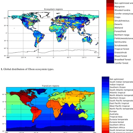
ao= −2 ‰, and is not optimized. The parametersλbandλo represent the linear scaling factors for each week and ecosys-tem region (ecoregion) to adjust the net carbon exchange over land and ocean surfaces, respectively. For land, the scal-ing factor is associated with one scalar per ecoregion based on the Olson (1985) land use classification following Peters et al. (2005, 2007) (Fig. 1). The terrestrial biosphere is fur-ther divided into 11 larger geographical areas also known as TransCom regions (Gurney et al., 2002). Like in the early CarbonTracker releases, each of the 11 TransCom land re-gions contains a maximum of 19 ecoregion types (Fig. 2) and the ocean is divided into 30 large basins encompassing large-scale ocean circulation features. This gives a maximum of 239 (=11·19+30) different scaling factors each week (Pe-ters et al., 2007). The new parameter isλdiscr, which is used to scale a maximum of 209 terrestrial discrimination param-eters per week. They are associated with the same 1◦×1◦ ecoregions as the terrestrial fluxes. Note that the maximum number of scalable land parameters is in reality∼130, and not 209, because not each land region contains all 19 ecore-gion types.
90° S 60° S 30° S 0° 30° N 60° N
180° 120° W 60° W 0° 60° E 120° E 180°
180° 180°
Ecosystem regions
Conifer forest Broadleaf forest Mixed forest Grass/shrub Tropical forest Scrub/woods Semitundra Fields/woods/savanna Northern taiga Forest/field Wetland Deserts Shrub/tree/suc. Crops Conifer snowy/coastal Wooded tundra Mangrove Non-optimized areas
Figure 1.Global distribution of Olson ecosystem types.
90° S 60° S 30° S 0° 30° N 60° N
180° 120° W 60° W 0° 60° E 120° E 180°
180° 180°
TransCom regions
North American boreal North American temperate South American tropical South American temperate Northern Africa Southern Africa Eurasia boreal Eurasia temperate Tropical Asia Australia Europe North Pacific temperate West Pacific tropical East Pacific tropical South Pacific temperate Northern Ocean North Atlantic temperate Atlantic tropical South Atlantic temperate Southern Ocean Indian tropical South Indian temperate Not optimized
Figure 2.Earth’s partitioning into 11 land regions and 11 ocean regions according to the TransCom project. The ocean regions are divided into 30 smaller basins (not shown) and the land regions can contain up to 19 different ecoregions as shown in Fig. 1.
in Sect. 3.2. The fossil fuel combustion, biomass burning, and terrestrial and ocean isodisequilibrium fluxes all remain fixed a priori estimates. We describe in Sect. 3.1 the tuning of the latter disequilibrium fluxes to close the long-term mean balance ofδ13C in our system.
The scaling factors λb, λo, and λdiscr are the unknowns that are combined in state vector x (with dimension s), for which we will try to find an optimal solution by minimizing a quadratic cost function. In this function, there is a balance between information drawn from the observation vector y (with dimension m) with a covarianceR(m×m) and prior
knowledge from the state vectorxp(s) with a covarianceP (s×s):
J=(y−H (x))T R−1(y−H (x))
+ x−xp
T
P−1 x−xp
. (6)
The solution forxthat minimizesJ is (Tarantola, 2005) x= xp+K·
y−H xp
, (7)
where Krepresents the Kalman gain matrix (Peters et al., 2005). Equation (7) can be expressed in terms ofλ (poste-rior scaling factor), λp (prior scaling factor), and separate
measurements of CO2(c) andδ13C (δ) with dimensions (j) and (k), respectively:
λbio1 . . λbio209 λoce210 . . λoce239 λdiscr240 . . λdiscr448 =
λpbio1
. . λpbio209
λpoce210
. . λpoce239
λpdiscr240
. . λpdiscr448
(8)
+K·
c1 c2 c3 c4 . . cj δ1 δ2 δ3 δ4 . . δk −H
λpbio1
. . λpbio209
λpoce210
. . λpoce239
λpdiscr240
. . λpdiscr448
.
In state vectors x andxp, the scaling factors for terrestrial discrimination are appended after the flux scaling factors. Similarly in the observation vectors yandH (xp), theδ13C observations are appended after the CO2observations. TheK matrix determines how much a scaling factor needs to change given a set of CO2andδ13C measurements. The matricesR
andPmodulate whether observations or bottom-up estimates are given more weight to the solution.
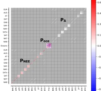
The P matrix contains 448×448 elements in total and is shown in Fig. 3. The first 209×209 element block con-tains the land flux uncertainties per ecoregion and their spa-tial correlations. The second 30×30 element block con-tains the ocean flux uncertainties per ocean basin. We gave the land scalars and the ocean scalars a maximum uncer-tainty of 80 and 100 % along the diagonal, respectively, as in earlier CarbonTracker releases. The third 209×209 el-ement block contains the terrestrial discrimination scalars with a maximum uncertainty of 20 % along the diagonal
with an identical spatial correlation structure as applied to the terrestrial flux uncertainty scalars. This implies that we can scaleph by a factor of 1.0±0.2, and thus for a typ-ical C3plant (ph= −20 ‰) the mean and uncertainty lies around −20±4 ‰. Furthermore, there is covariation be-tween ecoregions of nearby TransCom regions, e.g., bebe-tween North America boreal and temperate regions and between Europe and Eurasian regions. We did not allow covariances between net exchange and discrimination in order to give the parameters enough freedom in the solution.
The covariance structure ofRis similar to CO2-only CT-DAS, but is extended with additional uncertainties inδ13C observations. These expected uncertainties quantify our abil-ity to simulate observations given the uncertainty in atmo-spheric transport modeling and measurement errors. Sec-tion 2.3.5 gives an overview of the used uncertainties for each observation category.
With this inversion framework in place CTDAS-C13 pro-gresses in a similar manner as the traditional CO2-only CT-DAS. For each week, the set of unknowns in the state vec-tor are updated in a cycle that contains two steps. First there is a forecast step, which is driven by our fluxes and current background state vectorxpto forecast an ensemble of CO2 and13CO2mole fractions 5 weeks ahead in time. This is fol-lowed by an analysis step to determine the new state of the system with Eq. (8) such that it is consistent with the obser-vations for the current week of the cycle. The analyzed state is propagated to the next cycle using the same model as Pe-ters et al. (2007, Eq. 1 of the Supplement), and with this new state a new cycle begins with another forecast step to forecast a new ensemble of the background state 5 weeks ahead in time, now with an additional set of observations from a new week. The ensemble for each tracer is created from 150 en-semble members to provide a Gaussian probability density function of the state vector.
The simulation of atmospheric transport is provided by the two-way nested global transport model TM5 release 3 (Krol et al., 2005). This application simulates the atmospheric transport of CO2and13CO2at a global 6◦×4◦ resolution, with no nesting. It is driven by 3 hourly meteorological out-put from ECMWF ERA-Interim reanalysis (Dee et al., 2011). All the CO2 and 13CO2 flux fields provided to the model are in units of mol CO2m−2s−1and mol13CO2m−2s−1, re-spectively. Atmospheric concentrations of CO2 and13CO2 are calculated as mole fractions in mol mol−1. Signatures of
δ13C are computed to the relative per mil value using the following conversion formulation in order to facilitate com-parison with observations:
δ13C=
R
Rref −1
·1000, (9)
P
NEEP
oceP
ΔFigure 3.The priorPcovariance structure represents squared uncertainty of the dimensionless state vector. The first 209×209 element block represents the covariance matrix for land NEE with a maximum diagonal uncertainty of 0.64 (equivalent to 80 %), the second 30×30 element block represents the covariance matrix for ocean fluxes with a maximum diagonal uncertainty of 1.0 (equivalent to 100 %), and the third 209×209 element block represents the covariance matrix for1phwith a maximum diagonal uncertainty of 0.04 (equivalent to 20 %). The matrix is organized according to TransCom ocean basins and land regions, where each land region contains 19 potential ecoregions (see Figs. 1 and 2).
2.3 Prior estimates and observations
2.3.1 Terrestrial biosphere fluxes
The terrestrial first-guess net CO2 exchange (Nb) and fire (Ffire) estimates were calculated in the Simple-Biosphere Carnegie–Ames–Stanford Approach model (SiB-CASA; Schaefer et al., 2008) on a 1◦×1◦grid on a 10 min time resolution and were further processed into 3 hourly mean fluxes to serve as input for CTDAS-C13. SiBCASA is a biogeochemical model that calculates carbon, isotope, water, and energy exchange fluxes. The model inherited the aerodynamic and surface resistance models from SiB (Sell-ers et al., 1996) to solve for CO2partial pressures in an iter-ative loop to acquire a balance between net assimilation rate, stomatal conductance, mesophyll conductance, and CO2 par-tial pressures. The aerodynamic resistance model describes the turbulent transfer processes using the Monin–Obuhkov similarity theory. The surface and interior resistance mod-els describe the pathway of CO2 (but also water and heat)
from the plant and soil is calculated in the CASA part of the model using 13 biogeochemical pools with environment-influenced turnover rates (Schaefer et al., 2008).
2.3.2 Ocean fluxes
The ocean first-guess net CO2exchange (No) estimates de-rive from ocean inversions from Jacobson et al. (2007). These long-term estimates are combined with the quadratic gas-transfer velocity from 3 hourly ECMWF ERA-Interim wind fields (Wanninkhof, 1992) to create fluxes on a 1◦×1◦grid at a 3 hourly temporal resolution. An additional trend was ap-plied to the fluxes to ensure that increases in anthropogenic uptake are proportional to increases in atmospheric CO2 lev-els (see http://www.esrl.noaa.gov/gmd/ccgg/carbontracker).
2.3.3 Fossil fuel emissions
Fossil fuel CO2 emissions (Fff) were made available on 1◦×1◦grid at a monthly temporal resolution. They are de-rived from a combination of databases: EDGAR4.2, CDIAC, and BP statistics (see http://www.esrl.noaa.gov/gmd/ccgg/ carbontracker).
2.3.4 Isotope and disequilibrium fluxes
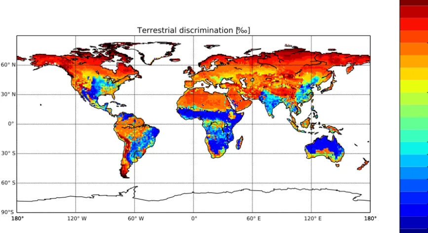
To calculate the fluxes of13CO2from land surfaces we used the photosynthetic discrimination parameterization (Eq. 2) for C3plants in the SiBCASA model (van der Velde et al., 2014). The weighted leaf-level value for C3discrimination is typically 19.0 ‰, and given the more efficient CO2bonding with the Rubisco enzyme, C4discrimination is 4.4 ‰ (Still et al., 2003; Suits et al., 2005). Given the dominance of C3 plant growth (70 % of global GPP), the global mean discrim-ination in SiBCASA has been estimated at 1ph=15.2 ‰. SiBCASA’s spatial heterogeneity of land discrimination is shown in Fig. 4. It reflects the land use distribution and the environmental forcing. Large discrimination values can be found in the temperate regions, the boreal forests, and in the humid environments such as the tropical rain forests in South America, Africa, and South East Asia. Small discrimination values can be found in the United States corn belt and in the dry climate regions such as the African savannas and Aus-tralian grasslands, where there is an abundance of C4plant growth. More subtle variations in 1ph in C3 dominant re-gions are driven by differences in environmental conditions (e.g., humidity, groundwater availability, and light intensity). Weekly 1◦×1◦fields for1phwere used to map the regular 3 hourly net CO2fluxes to13CO2fluxes:
[terrestrial net13C exchange term] =
λbNb λdiscrph/1000+1Ra, (10) wherephis derived from SiBCASA’s1ph output. Their re-lation is straightforward
ph= −1ph. (11)
For the calculation of 13CO2 biomass burning flux we as-sumedRfireto be very close to the signature of newly assim-ilated photosynthates:
13F
fire=Ffire λdiscrph/1000+1Ra. (12) The 13CO
2 fossil fuel emissions are calculated with Rff= 0.0107786, given that the global mean value ofδffis equal to −30 ‰:
13F
ff=FffRff. (13)
Note that we did not vary δff for different fuel types in this version of CTDAS-C13, but such variability could be included in the future based on the work of Andres et al. (2000).
The ocean discrimination parameteraois assumed to be constant at−2 ‰ as in many comparable studies (e.g., Tans et al., 1993; Ciais et al., 1995; Alden et al., 2010), and is not optimized. The regular 3 hourly net CO2fluxes were mapped to13CO2fluxes as follows:
[ocean net13C exchange term] =λoNo(ao/1000+1) Ra, (14) The isodisequilibrium fluxes (Db and Do, in mol13CO2m−2s−1) were made available on a monthly 1◦×1◦resolution.Dbis calculated using SiBCASA’s gross natural respiratory flux scaled with isotopic disequilibrium of the terrestrial biosphere with the current atmosphere, i.e.,
Fba δb−δbeq. Because fossil fuel emissions add isotopically depleted CO2 to the atmosphere, the biosphere signature
δbfollows with a time lag dependent on the residence time of carbon in the vegetation and soils. That implies δb is larger thanδeqb , which is the biosphere signature that is in equilibrium with the current atmosphere (Tans et al., 1993).
Dbhas a positive tendency on atmospheric δ13C as carbon originating from different SiBCASA pools is older and more enriched in13C than the isotopic signature of recently fixed photosynthates. The SiBCASA pool configuration is described in detail in van der Velde et al. (2014).
Dois calculated from the outgassing flux of CO2 scaled with the isotopic disequilibrium of the ocean surface with the current atmosphere, i.e.,Foa δeqa −δa. Theδaeq term is determined from a global network ofδ13C measurements in dissolved inorganic carbon (Gruber et al., 1999).Foais pa-rameterized as a function of surface ocean partial pressure of CO2and wind speed after Takahashi et al. (2009). Wind speed and solubility are assumed to remain constant year-to-year. The disequilibrium fluxes are positive from the equator to approximately 60◦ of latitude in both directions and are negative beyond that.
2.3.5 Observations
90°S 60° S 30° S 0° 30° N 60° N
180° 120° W 60° W 0° 60° E 120° E 180°
180° 180°
Terrestrial discrimination [ ]
0 2 4 6 8 10 12 14 16 18 20 22
Figure 4.Mean (2001–2011) modeled discrimination parameter1ph(‰) from SiBCASA. The discrimination is more detailed for1ph> 16 ‰ to highlight the more subtle variations in1phin the dominant C3regions that experience different environmental forcing.
products that include the provider’s original data and meta-data reformatted into the ObsPack framework (Masarie et al., 2014).
From the available CO2 observations, approximately 24 000 weekly flask measurements were used in the assimi-lation from a fixed network of 58 surface sites. Another large set of 174 000 measurements came from 23 semi-continuous in situ sites. Most CO2 measurements are obtained with a nominal precision of±0.1 ppm. The remainder of sites and measurements (including from aircraft or shipboard) were not used because of double records, and some measure-ments were kept for independent checks. A small fraction was omitted as our model could not resolve certain locations at a coarse resolution.
For the dual-species inversions we also used 22 000 flask measurements ofδ13C from 53 different surface sites. A fur-ther 5600 measurements from five different sites were ob-tained using programmable flask packages, which measure
δ13C at a daily resolution. The isotope ratios are measured by dual inlet mass spectrometry with a precision of±0.01 ‰.
We determined observation uncertainties (model–data mismatch or MDM) for each of theδ13C measurement sites in a heuristic manner based on earlier test inversions. These values are added to the diagonal of R. A too small error would give an unrealistic amount of confidence how well the model is expected to represent the measurement location during sampling but a too large error would give very little confidence to the measurement representation.
Table 1.Summary of assignedδ13C model–data mismatch (MDM), the category-averaged and 1σSD of the innovationχ2, and number of sites per category.
Site category MDM (‰) χ2 No. of sites
land 0.13 0.97±0.52 10
mixed 0.080 0.80±0.34 11
marine boundary layer 0.03 1.29±0.70 15 deep Southern 0.03 1.22±0.44 07 Hemisphere
problem 0.4 0.63±0.48 10
Figure 5.Annual mean carbon (xaxis) andδ13C (yaxis) growth rates for(a)the prior estimates and for(b)the NEW−CO2C13 experiment. Colored arrows represent the different sources and sinks of the carbon cycle. A closed budget for both tracers was accomplished in the NEW−CO2C13 experiment, as indicated by the resultant vector (sum of all colored arrows) returning to the black arrow (observed growth rate in atmosphere). To close the long-term trend we increased the isodisequilibrium fluxes by 20 %.
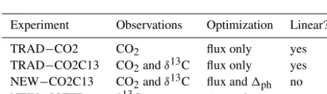
Table 2.Summary of the four inversion experiments, the observa-tions used, the optimized items (ocean and land fluxes, and1ph), and their linearity. The prefix TRAD−refers to traditional, i.e., ex-periments that have been performed in the past in any way, shape or form. The prefix NEW−refers to a new type of inversions used in this publication. NEW−CO2C13 used the default CTDAS-C13 model setup as described in the Methodology, while NEW−2STEP solved for1phusing onlyδ13C data.
Experiment Observations Optimization Linear?
TRAD−CO2 CO2 flux only yes
TRAD−CO2C13 CO2andδ13C flux only yes NEW−CO2C13 CO2andδ13C flux and1ph no
NEW−2STEP δ13C 1phonly yes
1.0. For the CO2measurement sites we used a similar set of MDM values as in previous CarbonTracker releases.
2.4 Experiments
We performed four inversion experiments as summarized in Table 2. The simulation period covered the years 2000 through 2011, but our analyses focused on the period 2001– 2011, i.e., we omitted the spin-up year. As a benchmark, we performed a traditional inversion to estimate the net carbon exchange fluxes of the ocean and land using only CO2 ob-servations, which we call TRAD−CO2. For the second in-version, we addedδ13C observations alongside CO2to con-strain only the exchange fluxes; therefore, we call this ex-periment TRAD−CO2C13. The experiment in which we es-timated discrimination and fluxes simultaneously is called NEW−CO2C13. This inversion is nonlinear because the dis-crimination scaling parameter is in the same multiplication term as the net flux scaling parameter. The fourth experiment was a linear inversion experiment where we estimated only the land discrimination parameter usingδ13C data. We call
this experiment NEW−2STEP because discrimination was solved in a second step after optimization of the net exchange fluxes. This means that ocean and land fluxes were derived from the optimized state vector and its covariance from the TRAD−CO2 inversion.
3 Results
3.1 Comparison to observations of CO2andδ13C from
the global network
We first evaluate the global CO2 andδ13C budgets simu-lated by our combination of fluxes as described in Sect. 2 to assess where we expect the largest changes in the opti-mization. As shown in Fig. 5a, the prior net exchange flux estimates and unscaled disequilibrium fluxes were not large enough to close the gap with the observed tracers, CO2, and
δ13C. The sum of the flux arrows overestimated the annual CO2 growth rate along the x axis and overestimatedδ13C depletion along they axis. In a traditional TRAD−CO2 in-version, the estimated ocean and land fluxes closed the CO2 budget along thex axis. The leverage in the net exchange fluxes was, however, not large enough to close theδ13C bud-get along the y axis as well. In an inversion that includes
of our inversions without creating unrealistic carbon sinks over land and oceans (Fig. 5b). Most importantly, closing the climatological (11 year) budget allowed us to focus our study on interannual changes in the net fluxes and photosynthetic discrimination.
We obtained the best fit with δ13C data when the land and ocean disequilibrium flux were scaled by a factor of 1.2 without changing either their spatial patterns or time trends. This is consistent with recent double deconvolution studies where the globalδ13C balance was closed with a factor of 1.3 in land and ocean disequilibrium (Alden et al., 2010). Our value was determined after assessing an ensemble of differ-ent sets of scaling numbers (ranging from 1.1 to 1.5) in a for-ward TM5 simulation, which was driven by the optimized net land and ocean flux estimates from the TRAD−CO2 experi-ment. This assured a closed multi-yearδ13C budget together with a closed multi-year CO2 budget. As selection criteria, we used (1) the 11 year mean root mean square difference (RMSD) of a large selection of δ13C sites and (2) the av-erage bias between simulated and observed values. In the non-scaled disequilibrium simulation we obtained a RMSD of 0.165 ‰ and a bias of−0.110 ‰ averaged over all sites. The optimal result was obtained with a scaling factor of 1.2, which reduced the RMSD to 0.079 ‰ and the mean bias to −0.010 ‰. Note that these scaling factors cannot be applied to other inversion studies because the disequilibrium scaling factors are tuned for this particular system and time period.
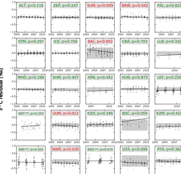
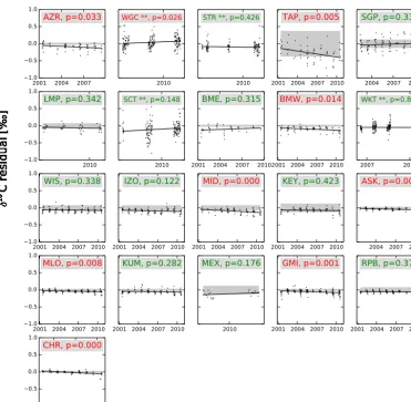
To demonstrate our procedure in terms of individual data sets, we refer to Fig. 6. After scaling the disequilibrium fluxes and using optimized net carbon exchange from the TRAD−CO2 inversion, time series of δ13C at 32 of the 46 Northern Hemisphere sites showed no remaining signifi-cant trend (sites wherepvalue>0.05) in the summer residu-als, and the residuals from the trend lines were within or close to the MDM specified for our dual-species inversions. Some of the sites with remaining trends are located at great dis-tances from large continental carbon sources and sinks, and exert little influence on the posterior λdiscr parameter (e.g., CHR, GMI). Some of the other sites were assigned a large MDM (e.g., BAL, NWR, TAP) giving them less weight in the estimation of the posteriorλdiscrparameter. The collection of sites with remaining trends do not seem to have a systematic geographic pattern and are likely reflecting a change in lo-cal oceanic or biospheric isotope exchange, such as must be the case for the Bermuda West (BMW, non-significant pos-itive trend) and Bermuda East (BME, significant downward trend) site.
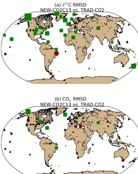
With the long-term trend of δ13C appropriately captured, we proceeded to optimize NEE and1phwith our new frame-work (NEW−CO2C13). We show that this inversion fur-ther reduced δ13C residuals (Fig. 7a), without compromis-ing (nor strongly improvcompromis-ing) the fit to CO2(Fig. 7b) that we attained from the TRAD−CO2 inversion. In Fig. 7a the ra-tio of δ13C RMSD of NEW−CO2C13 to δ13C RMSD of the TRAD−CO2 inversions was at most sites smaller or
equal to 0.95 (indicating a significantly higher accuracy of NEW−CO2C13 in form of bias and noise reduction):
δ13C RMSD(NEW−CO2C13) δ13C RMSD(TRAD−CO2) <0.95.
In Fig. 7b, the ratio of CO2RMSD of NEW−CO2C13 to CO2RMSD of TRAD−CO2 was at most locations between 0.95 and 1.05. This suggests that the two atmospheric con-straints applied are complementary, and there is no indica-tion that the TRAD−CO2 results from CarbonTracker were inconsistent withδ13C measurements. This is an important prerequisite for a credible estimate of discrimination in our system. Furthermore, Fig. 7a shows a notable latitudinal di-vide in the reduction ofδ13C RMSD, indicating the utility of NEW−CO2C13 in the Northern Hemisphere due to the large availability of measurements and scalable discrimination pa-rameters.
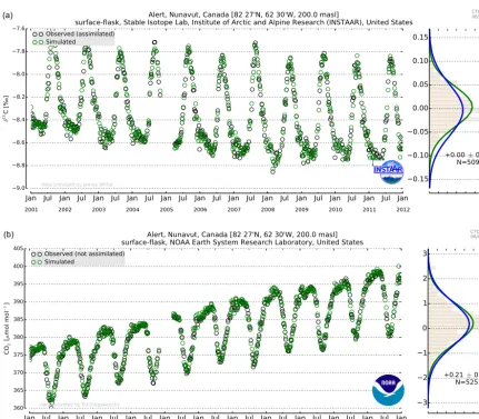
At sites like Alert (Nunavut, Canada) the NEW−CO2C13 inversion provided a better fit to the measured data than the TRAD−CO2 inversion (Fig. 8). The 11 year averagedδ13C residuals were close to zero for both inversions, as the dise-quilibrium flux was tuned specifically to prevent large resid-uals in a-priori simulatedδ13C as described in Sect. 3.1. The 1σ SD of the δ13C residuals at Alert were smaller in the NEW−CO2C13 inversion in comparison to TRAD−CO2 due to the additional optimization of1ph alongside net ex-change fluxes. The CO2residuals for Alert in Fig. 8 were for both inversions almost identical.
3.2 Linear and nonlinear estimates of net carbon uptake and land discrimination
Simultaneously optimizing bothλdiscrandλbiois inherently nonlinear and thus possibly problematic for our assimilation system; therefore, we tested the validity of our approach in the NEW−CO2C13 inversion. We hypothesized that a re-gion’s net carbon uptake and discrimination would change in a similar fashion in the nonlinear inversion, as it would for a linear inversion. The linear inversion experiment consisted of two consecutive steps: (1) the optimization of the net ex-change fluxes using only CO2 observations (TRAD−CO2) followed by (2) the estimation of the land discrimination pa-rameter using only δ13C observations (NEW−2STEP). In the nonlinear NEW−CO2C13 inversion the optimization of fluxes and discrimination was done simultaneously. For net carbon uptake by vegetation, we refer to net ecosystem ex-change or NEE defined as positive when CO2 is taken up from the atmosphere. For plant isotope discrimination we re-fer to1phin per mil, which is defined as positive.
ag-Figure 6.
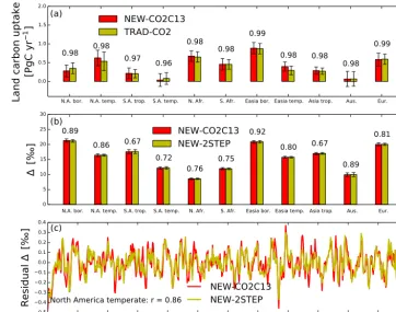
gregated 1ph values. In the boreal regions, where there is very little C4plant growth, the discrimination is at its max-imum (approximately 20 ‰, 5 ‰ above the global average), but in regions where there is C4 plant growth (e.g., due to agriculture in the United States or savannas in Africa) the mean 1ph values are lower (approximately 12–15 ‰). These regional patterns of1ph imposed by SiBCASA (see also Fig. 4) are maintained by the NEW−CO2C13 inversion framework. Because we aimed to retrieve robust temporal patterns of IAV, the most relevant indicators for the robust-ness of our nonlinear inversion approach are given by the cor-relation coefficients (r) between the two types of inversions. We calculated r for NEE and 1ph between the linear and nonlinear inversions. As the seasonal cycles in uptake and discrimination are largely dictated by the prior estimates, we removed them using a 3 month boxcar mean smooth curve fitting to obtain the anomalies relative to the seasonal trend. The NEE in NEW−CO2C13 is very similar to the NEE in TRAD−CO2, as indicated by the highr values (>0.96 for
N=52·11 weeks) for all TransCom regions. Ther values are lower for1ph, but still exceed 0.75 in the Northern
Hemi-sphere. The correlation is particularly high over North Amer-ica boreal, North AmerAmer-ica temperate, and European regions. Smaller correlations are obtained in tropical and temperate South America and tropical Asia. This is expected, however, as these regions typically suffer from a lack of observational constraints.
esti-Figure 6.Summer (JJA) residuals ofδ13C (‰) in CO2for 46 sites (excluding aircraft and ships) situated in the Northern Hemisphere. These sites are ordered based on the their latitudinal location; most northern site is placed at the top left (Alert, Canada) and the site nearest to the equator at the bottom left in the second part of Fig. 6 (Christmas Island, Republic of Kiribati). All residuals (simulated minus observed) are calculated from a traditional TRAD−CO2 inversion with scaled disequilibrium fluxes. Assuming a closed long-term mean budget in δ13C, we tested the null hypothesis that the slope of the linear regression line is zero. Sites with a trend where thep value is smaller than the significance level of 5 % are shown in red, whereas the remaining sites without significant trend are shown in green. The sample uncertainty (model–data mismatch) used for the NEW−CO2C13 and NEW−2STEP inversions is displayed by transparent gray areas. Sites marked with ** were not included in the inversions but were used for independent verification. For detailed information of the sites and their locations, we refer to the NOAA website: http://www.esrl.noaa.gov/gmd/ccgg/carbontracker/observations.php.
Table 3.Northern Hemisphere land net carbon uptake (NEE, (Pg C yr−1)) and land discrimination (1ph, (‰)) 11 year mean estimates, and IAV (±1σSD) from SiBCASA (prior) and the four inversion experiments. The last row gives the correlation coefficientrbetween 11 annual mean NEE and1phvalues.
Prior TRAD−CO2 TRAD−CO2C13 NEW−CO2C13 NEW−2STEP
NEE 0.22±0.28 2.44±0.46 2.65±0.49 2.58±0.46 2.44±0.46
1ph 18.1±0.02 18.1±0.02 18.1±0.02 18.2±0.17 18.3±0.17
r −0.26 −0.14 −0.18 0.79 0.78
mate, to estimate NEE but not 1ph. The SiBCASA terres-trial biosphere model that provides the first-guess NEE and
1phof our data assimilation framework based on commonly
Figure 7.A comparison of the relative performance of inversion techniques for the period 2001 through 2006 based on the ratio of the model–data(a)δ13C root mean square difference (RMSD) of NEW−CO2C13 toδ13C RMSD of TRAD−CO2, and(b)CO2 RMSD of NEW−CO2C13 to CO2RMSD of the TRAD−CO2 in-version. A ratio lower than 1.0 indicates a higher accuracy of the NEW−CO2C13 inversion technique; green sites indicate a ratio less than or equal to 0.95, red sites indicate a ratio greater than or equal to 1.05, and sites where the difference in respective RMSD is less than 0.05 are given in black. The size of each symbol is a mea-sure of the relative performance of NEW−CO2C13 in comparison to TRAD−CO2. The larger the symbol the more the ratio of RMSD differs from 1.0.
1phand the correlation with NEE were driven byδ13C obser-vations, and were not a symptom of the systems inability to separately estimate NEE and 1ph variations. This suggests that the estimated IAV of 1ph in the nonlinear inversion is truly a signal retrieved fromδ13C that would otherwise be aliased erroneously into the carbon fluxes or not retrieved at all.
3.3 Independent verification with drought indices
A closer inspection reveals that the reported correlation be-tween the Northern Hemisphere’s NEE and1ph in Table 3 could indicate a moisture-driven response on the ecosys-tem level. We identified several moments of severe to ex-treme drought as characterized by the Standardized Precipi-tation and Evaporation Index (SPEI; Vicente-Serrano et al.,
2010) below−1.0 that covered an extensive area of more than a million square kilometers in the United States. These droughts are described in literature as the droughts (or heat waves) of summer 2002 (Seager, 2010; Schwalm et al., 2012) and 2011 (Long et al., 2013). The annual averaged maps of SPEI for 2001–2011 are shown in the top panel of Fig. 10 cal-culated for the Northern American temperate TransCom do-main. Independent of the SPEI drought index, we estimated changes in1ph and NEE over the same American domain with the NEW−CO2C13 inversion using atmospheric CO2 andδ13C data (Fig. 10 middle and lower panels). A corre-lation between1ph and SPEI could only be established by applying an area weighting function to the SPEI index to give years that experienced large and severe droughts, the strongest association with reductions in1ph. We used the following function for the Weighted Drought Index (WDI): WDI =
P
i=1(SPEI[i] · Grid-cell-area[i])
Total-area .
In words, we sum over the product of the SPEI index and the grid cell surface area where SPEI is below−1.0 and sub-sequently we divide it by the total area of the TransCom do-main. Hence, the WDI is an expression of the drought in terms of the surface area that is affected. A larger drought surface area will result in a more negative WDI. Using this function, we see that the lower values for1ph correspond strongly with years of low SPEI over large serried areas, indi-cating a temporal correlation ofr= +0.75 between the SPEI variable and1ph (see correlation in Fig. 11 with a signif-icant slope: p=0.008, 95 % confidence interval of a two-sided distribution with 9 degrees of freedom). The two largest anomalies (>1σ of 11 year IAV) in annual mean1ph corre-spond with low SPEI in 2002 and in 2011. A third notable drought as recorded in SPEI happened in 2006; although car-bon uptake was reduced, it did not amount to a significant signal in1ph. Similar correlations do exist over other parts of the Northern Hemisphere in our inversion solution. For in-stance, severe droughts in western Europe (2003) and Russia (2010) lowered the discrimination by 1.0 ‰, and exceeded more than 1σ SD of its 11 year IAV (not shown).
In addition, in years when 1ph is low, the annual mean NEE tends to be low too, possibly as a result of reduced GPP. This implies that leaf stomata have partially closed and are therefore affecting both1ph and carbon uptake from pho-tosynthesis. The reduction of the optimized net carbon sink for North America is 100–400 Tg C yr−1during the drought years of 2002, 2006, and 2011 (in comparison to their sur-rounding years).
(a)
(b)
Figure 8.Comparison of two different inversion experiments at Alert (ALT, Canada). The top panel displaysδ13C observations (black circles) together with simulatedδ13C from NEW−CO2C13 (green circles). The top right panel displays the probability density functions (PDFs) of the residuals between NEW−CO2C13 and observed (green) and between TRAD−CO2 and observed (blue). The lower panel displays independent flask measurements (not used in the assimilation) of CO2(black circles) at Alert with simulated CO2from NEW−CO2C13 (green circles). Notice the almost identical distribution of the residual PDFs between NEW−CO2C13 and TRAD−CO2 inversion techniques.
where the drought index was negative over the mountain states, the impact on the carbon cycle was strongest over the eastern forests of the United States. In these forest ecosys-tems, CO2 exchange is much stronger than over the moun-tains, and hence their impact on atmosphericδ13C as well.
Notice that the prior net carbon sink is underestimated in comparison to the optimization because SiBCASA as-sumes a near steady state between GPP and TER (Fig. 10). SiBCASA was in fact able to simulate small carbon uptake anomalies during the reported droughts using its own envi-ronmental response parameterizations. However, it lacked a substantial amount of interannual variability in NEE and1ph and lacked a strong correlation of1phwith SPEI (Fig. 11). This suggests a potential absence of an important coupling between the hydrology and carbon discrimination processes in the model.
4 Discussion and conclusions
N.A. bor. N.A. temp. S.A. trop. S.A. temp. N. Afr. S. Afr. Easia bor. Easia temp. Asia trop. Aus. Eur. 0.0
0.5 1.0 1.5 2.0
Land carbon uptake
[P
g
C
y
r
−
1]
0.98 0.98 0.97
0.96 0.98
0.98 0.99
0.98 0.98 0.98
0.99 NEW-CO2C13
TRAD-CO2
0 5 10 15 20 25 30
∆
[
]
0.89
0.86 0.67 0.72
0.76 0.75
0.92
0.80 0.67
0.89 0.81 NEW-CO2C13
NEW-2STEP
Jan '01 Jan '02 Jan '03 Jan '04 Jan '05 Jan '06 Jan '07 Jan '08 Jan '09 Jan '10 Jan '11 0.5
0.4 0.3 0.2 0.1 0.0 0.1 0.2 0.3 0.4
R
e
si
d
u
a
l
∆
[
]
North America temperate: r = 0.86
NEW-CO2C13 NEW-2STEP
N.A. bor. N.A. temp. S.A. trop. S.A. temp. N. Afr. S. Afr. Easia bor. Easia temp. Asia trop. Aus. Eur.
(a)
(b)
(c)
Figure 9. (a)the 11 year mean land carbon uptake (Pg C yr−1) for each TransCom region with estimates from the nonlinear NEW−CO2C13 inversion (red) and estimates from the linear TRAD−CO2 inversion (yellow). Error bars depict 1σ SD of the flux IAV. The 11 year corre-lation coefficientsr between the two inversion methods are given on top of the bars. These correlations are based on the 3 month boxcar mean anomalies after subtracting the seasonal cycle. (b)Comparison of1ph (‰) between the NEW−CO2C13 inversion and the linear NEW−2STEP inversion. We again provide IAV error bars and correlation coefficients between inversion methods.(c)The 3 month boxcar mean anomalies in1phfor the North America temperate TransCom region to illustrate the high degree of similarity between both inversion methods (r=0.86).
0.50 0.45 0.40 0.35 0.30 0.25 0.20 0.15 0.10 0.05 Weighted drought index
15.8 16.0 16.2 16.4 16.6 16.8
Isotopic discrimination
[
]
Prior y = ax+b
a = 0.14, b = 16.05 r = +0.31, p = 0.348, N = 11
Optimized y = ax+b
a = 1.61, b = 16.75 r = +0.75, p = 0.008, N = 11
Figure 11. Weighted SPEI drought index (WDI) versus annual mean isotopic discrimination1ph integrated over the North American temperate domain. Results from the SiBCASA biosphere model (blue circles) show no significant correlation between1phand large-scale droughts, while the simultaneous optimization of carbon sinks and1phwith atmospheric CO2andδ13C observations (red triangles) suggests a highly significant correlation can be derived. The slope of the red regression line is 1.61 ‰/WDI (p=0.008, 95% confidence interval of a two-sided distribution with 9 degrees of freedom). The SiBCASA slope is, however, not significantly different from zero (p0.05). The integrated1phvalues are GPP-weighted per grid box as in Fig. 10. WDI is based on the SPEI index but area weighted to give years with large serried areas that experienced severe droughts (with SPEI smaller than−1.2) more leverage.
the effects of IAV on the strength of photosynthesis over C3 and C4 vegetation; (b) the variations in mesophyll conduc-tance are not expected to vary much from year-to-year, such as ecosystem composition; or (c) the variations in mesophyll conductance would enhance the intercellular CO2levels (and thus1ph) rather than reduce it, such as increased radiance of the leaves under reduced cloud cover. This suggests the pos-sibility that the impact of environmental stress on stomatal conductance and carbon uptake is much larger than currently simulated by the widely used drought parameterizations in terrestrial biosphere models. These parameterizations are of-ten derived from laboratory observations or plot-scale obser-vations that often aggregate poorly over much larger scales. Our first results suggest that a data assimilation system that uses the global atmosphericδ13C record, in concert with the CO2 record, can offer new insights on large-scale drought dynamics of the coupled vegetation–atmosphere system.
It is unlikely that our terrestrial biosphere model will reproduce the new large-scale atmospheric constraints on NEE and 1ph with a simple adjustment of the currently used drought response parameterizations (such as stomatal conductance and soil water stress inhibition functions). We experimented with a different stomatal conductance model based on vapor pressure deficit (VPD; Leuning, 1995) rather than relative humidity as it was shown to better predict changes in the isotopic composition in tree rings (Ballantyne et al., 2010). This modification, however, did not change the
variability in simulated atmospheric δ13C found in van der Velde et al. (2013) could well be (partially) ascribed to the lack of sensitivity towards soil moisture stress in SiBCASA. There is also evidence that the conventional use of land cover types in biosphere models does not adequately describe the spatial variations in carbon exchange (Bloom et al., 2016).
As with any data assimilation system, the number of avail-able observations largely determines the assimilation sys-tem’s ability to retrieve meaningful signals. Our current method relies on atmospheric δ13C anomalies that affect multiple monitoring sites at the same time due to low signal-to-noise ratios at each site, but the network coverage over many parts of the world is still sparse. The increase in the number of measurement sites, and the addition of δ13C to many existing ones, particularly in sparsely populated ar-eas could benefit CTDAS-C13 greatly. New mar-easurement efforts are currently underway to improve our observational coverage in these sparsely sampled areas. Regular measure-ments of CO2 from aircraft vertical profiles have recently commenced at four different sites above the Amazon. These data have provided new insights on the carbon cycle under drought conditions (Gatti et al., 2014). These new measure-ments were successfully used in an application of CTDAS (van der Laan-Luijkx et al., 2015) and confirmed that the Amazonian CO2 uptake by vegetation was indeed reduced during the severe 2010 drought. Furthermore, some coau-thors are currently involved in a new collaborative effort to provide the first high-precision measurements of δ13C and other isotopes in CO2 from a large number of air samples collected over the Amazon basin. Using an assimilation sys-tem similar to that described here, these data would bolster our ability to quantify seasonal to interannual changes in the Amazonian carbon balance and better understand the influ-ence of drought stress on NEE.
The retrieved correlation between NEE and 1ph in the Northern Hemisphere was derived from atmospheric δ13C observations through our new dual-species approach, and thereby provided new insights on the land–atmosphere cou-pling of water and carbon on continental and hemispheric scales. The unconstrained SiBCASA model does not show a large enough response to drought both in terms of NEE and 1ph. The correlation between droughts and 1ph over the North American temperate domain (Fig. 10) can only be demonstrated after optimizing NEE and1phby applying at-mosphericδ13C and CO2constraints together. We emphasize that the reported correlations remain robust and significant even when changing the atmospheric transport characteris-tics (i.e., convection fields from ECMWF ERA-Interim me-teorology vs. default TM5 convection scheme), the optimiza-tion method (nonlinear vs. linear 2-step), and when changing the assumed model–data errors of our data assimilation sys-tem.
A potential problem with the current framework is that we cannot account for changes in the terrestrial isodisequi-librium flux. In Eq. (1), we forced all missing isotopic
vari-ability into termNbph without considering additional vari-ability from the isodisequilibrium term. Photosynthetic dis-crimination is also responsible for a portion of the variability in the terrestrial isodisequilibrium flux (van der Velde et al., 2013), but the extent is hard to quantify. Theδbeqsignature (i.e., the biosphere signature that is in equilibrium with the atmosphere) is a function of the current δa and 1ph, two quantities that ultimately exert influence on δb as the iso-topic signal carries through the series of carbon reservoirs (i.e., leaves, stems, roots, and ultimately the soils). The ab-sence of direct adjustments to the disequilibrium flux could mean we aliased erroneously isotopic signals only onto the net flux term of the budget. In light of recent observational evidence, the variability in the disequilibrium term might be of more importance than recently thought. Bowling et al. (2014) showed withδameasurements that the disequilibrium flux can become negative locally due to humidity-induced changes in1ph. We found that these effects on the1ph esti-mate are likely small mainly because gross flux variability is fundamentally limited and dampened by the large reservoir sizes from which it comes. In an experiment with SiBCASA where we allowed extra uncertainty in respiration and1phto drive through the disequilibrium isoflux we indeed found an increase in variability in the disequilibrium term, necessitat-ing 10 % less1ph variability to keep a closedδ13C budget. This indicates that allowing for errors in the disequilibrium fluxes, the variations in the estimated1ph parameter might be slightly smaller or larger than estimated with CTDAS-C13, but nonetheless still twice as large than estimated with SiBCASA. On one hand, using a more simplified but phys-ically consistent set of equations only based on gross fluxes (GPP and TER) to express the rate of change ofδa would eliminate the need for a disequilibrium term. On the other hand, this would complicate the closing of the CO2budget as it necessitates a way to effectively separate these two gross fluxes.
It is worth mentioning that the carbon residence time in land ecosystems is highly uncertain, and therefore the gross CO2 exchange as well. Welp et al. (2011) suggested that the current popular estimate of global GPP of 120 Pg C yr−1, which is also predicted by SiBCASA, may be a lower limit and could in reality be as large as 175 Pg C yr−1 to reflect faster turnover of carbon in the vegetation and soils. Such uncertainties were also underlined by Carvalhais et al. (2014) who found that higher precipitation rates are associated with faster carbon turnover, but that global modeled turnover is in fact often underestimated. We make a cautious conjecture that if GPP is in fact as large as claimed by Welp et al. (2011), and heterotrophic respiration is large too, it will partly ex-plain the current underestimation in the modeled disequilib-rium fluxes, which are a function of TER and ocean CO2 out-gassing. In this study, we closed the gap with a predetermined scaling factor of 1.2 on the disequilibrium fluxes for oceans and land without assuming actual changes in GPP, TER, or
as-similation system where we are using atmospheric data to si-multaneously optimize for terrestrial model parameters that exert an influence on GPP, TER, and carbon turnover. The CTDAS modular design (van der Laan-Luijkx et al., 2017) makes it now more straightforward to develop and implement such additional improvements.
To conclude, this study showed there is significant poten-tial to use atmospheric CO2andδ13C data as constraints on plant NEE and isotopic discrimination using a dual-species assimilation platform. Signals that would otherwise be lost in a single tracer data assimilation system, such as the possibil-ity of a drought-driven covariation between isotope discrim-ination and NEE or the separation of GPP from NEE, can potentially be detected in the described dual-species appli-cation of CTDAS. Continued and additional measurements of atmosphericδ13C and CO2, especially in future assimila-tion systems where biosphere model parameters are directly optimized, should help us better understand the hydrologi-cal and biogeochemihydrologi-cal interactions between the atmosphere and vegetation.
Code availability. The CTDAS-C13 and TM5 source code are made available online (ftp://ftp.cmdl.noaa.gov/user/ivar/CTDAS_ C13_sourcecode) (NOAA, 2018). More detailed model descriptions and information to run the code are available on the following web-sites: http://www.carbontracker.eu and http://tm.knmi.nl/index.php/ Main_Page.
Author contributions. IvdV, WP, and JM designed the study. IvdV, KS, WP, and MvdM built the inverse and forward modeling frame-works. PT, BV, and JW were responsible for theδ13C and CO2 measurement program. IvdV performed the analysis and wrote the main text. All authors gave input on the final manuscript.
Competing interests. The authors declare that they have no conflict of interest.
Acknowledgements. This study was financially supported by the Netherlands Organization for Scientific Research (NWO-VIDI: 864.08.012), by the Visiting Fellows Program of the Cooperative Institute for Research in Environmental Sciences, and by the National Computing Facilities Foundation (NCF project SH-060) for the use of supercomputing facilities.
Edited by: Alexander Archibald
Reviewed by: Peter Rayner and one anonymous referee
References
Alden, C. B., Miller, J. B., and White, J. W. C.: Can bottom-up ocean CO2 fluxes be reconciled with atmospheric 13C obser-vations?, Tellus B, 62, 369–388, https://doi.org/10.1111/j.1600-0889.2010.00481.x, 2010.
Andres, R. J., Marland, G., Boden, T. A., and Bischof, S.: Carbon dioxide emissions from fossil fuel consumption and cement man-ufacture, 1751–1991, and an estimate of their isotopic composi-tion and latitudinal distribucomposi-tion, in: The Carbon Cycle, edited by: Wigley, T. and Schimel, D., Cambridge University Press, Cam-bridge, UK,53–62, 2000.
Ball, J. T.: An analysis of stomatal conductance, Ph. D. thesis, Stan-ford University, StanStan-ford, CA, US, 1988.
Ballantyne, A. P., Miller, J. B., and Tans, P. P.: Apparent seasonal cycle in isotopic discrimination of carbon in the atmosphere and biosphere due to vapor pressure deficit, Global Biogeochem. Cy., 24, GB3018, https://doi.org/10.1029/2009GB003623, 2010. Basu, S., Miller, J. B., and Lehman, S.: Separation of biospheric
and fossil fuel fluxes of CO2by atmospheric inversion of CO2 and14CO2measurements: Observation System Simulations, At-mos. Chem. Phys., 16, 5665–5683, https://doi.org/10.5194/acp-16-5665-2016, 2016.
Bloom, A. A., Exbrayat, J.-F., van der Velde, I. R., Feng, L., and Williams, M.: The decadal state of the terrestrial carbon cycle: global retrievals of terrestrial carbon allocation, pools, and resi-dence times, P. Natl. Acad. Sci. USA, 113, 1285–1290, 2016. Booth, B. B., Jones, C. D., Collins, M., Totterdell, I. J.,
Cox, P. M., Sitch, S., Huntingford, C., Betts, R. A., Harris, G. R., and Lloyd, J.: High sensitivity of future global warming to land carbon cycle processes, Environ. Res. Lett., 7, 024002, https://doi.org/10.1088/1748-9326/7/2/024002, 2012.
Bowling, D. R., Ballantyne, A. P., Miller, J. B., Burns, S. P., Con-way, T. J., Menzer, O., Stephens, B. B., and Vaughn, B. H.: Ecological processes dominate the13C land disequilibrium in a Rocky Mountain subalpine forest, Global Biogeochem. Cy., 28, 352–370, https://doi.org/10.1002/2013GB004686, 2014. Bozhinova, D., van der Molen, M. K., van der Velde, I. R.,
Krol, M. C., van der Laan, S., Meijer, H. A. J., and Pe-ters, W.: Simulating the integrated summertime114CO2 sig-nature from anthropogenic emissions over Western Europe, At-mos. Chem. Phys., 14, 7273–7290, https://doi.org/10.5194/acp-14-7273-2014, 2014.
Bruhwiler, L., Dlugokencky, E., Masarie, K., Ishizawa, M., An-drews, A., Miller, J., Sweeney, C., Tans, P., and Worthy, D.: CarbonTracker-CH4: an assimilation system for estimating emis-sions of atmospheric methane, Atmos. Chem. Phys., 14, 8269– 8293, https://doi.org/10.5194/acp-14-8269-2014, 2014. Carvalhais, N., Forkel, M., Khomik, M., Bellarby, J., Jung, M.,
Migliavacca, M., Mu, M., Saatchi, S., Santoro, M., Thurner, M., Weber, U., Ahrens, B., Beer, C., Cescatti, A., Randerson, J. T., and Reichstein, M.: Global covariation of carbon turnover times with climate in terrestrial ecosystems, Nature, 514, 213–217, 2014.