ISSN: 1992-8645 www.jatit.org E-ISSN: 1817-3195
285
MODELLING OF BIOGAS PRODUCTION FROM
BANANA STEM WASTE WITH NEURAL NETWORKS
LEARNING STRATEGIES TO OPTIMSE THE
PRODUCTION
1
ABDUL SAHLI FAKHARUDIN, 2MD NASIR SULAIMAN, 2NORWATI MUSTAPHA 1
Faculty of Computer Systems and Software Engineering, University Malaysia Pahang, Gambang, Pahang, Malaysia.
2
Department of Computer Science, Faculty of Computer Science and Information Technology, University Putra Malaysia, Serdang, Selangor, Malaysia.
E-mail: [email protected], [email protected]
ABSTRACT
Biogas production from waste is a valuable renewable energy and with better process design, maximum biogas yield can be obtained from the same amount of waste. Modelling and optimisation are widely used in biological and chemical process domain to increase and to improve the efficiency of this process. In recent years, intelligence computation is applied to design a better process model and optimised biogas yield. This paper presents a comparative study of several neural networks learning (back-propagation, resilient propagation, Lavenberg-Marquardt and particle swarm optimisation) algorithms for process modelling and optimisation and its relation with the optimisation result. The result shows an improvement of around 10% of biogas production and 8% more from the engineering mathematical optimisation. Two main complications were identified, first one is the high accuracy modelling is not a guarantee for optimised production and the second is a false solution with high optimised production may happen. To clarify this situation, a solution is suggested using factor deviation percentage.
Keywords: Modelling, Optimisation, Neural Networks, Genetic Algorithms, Biogas
1. INTRODUCTION
The interest in converting biomass resources to an alternative fuel such as biogas, is receiving more attention in recent times [1]. The biogas yield can be improved with better process
design through modelling, simulation and
optimisation as an integrated part of modern design practice [2]. The mathematical modelling and optimisation of a chemical process were studied to ensure the process can be fully analysed and optimised for large production purposes in wide variety of field including energy [3], food industry [4] and medical engineering [5].
There were several studies on the application of intelligence computation and machine learning in exchange of the mathematical and statistical methods [6][7]. Artificial neural networks (ANN) and genetic algorithms (GA) were used in tandem to model, simulate and optimise the engineering process. The main capabilities of ANN as a pattern recognition system were utilised to generate the model. The prediction model was
being optimised using genetic algorithms to find the optimal yield based on heuristic search inspired by brain functions.
[8] used ANN modelling to predict the methane percentage in biogas recovered from landfill. The networks consist of 2 input nodes, 15 hidden nodes and one output node. The best mean
absolute percentage is 2.1075 with R2 of 0.8795.
The study of modelling on large anaerobic digester producing biogas from cattle waste using ANN by [9] was modelled using networks consist of 6 input neuron, 10 neurons each on 2 hidden layers and one output node. The networks were trained using a number of training algorithms available in Matlab and achieved a very low mean square errors (MSE)
values and high R2 values between 0.82 and 0.93.
ISSN: 1992-8645 www.jatit.org E-ISSN: 1817-3195
286 The findings of [6] presented the best ANN model was using 2 hidden neurons with 5 inputs and 1 output neuron in their study. The accuracy was measured using MSE around 6 × 10⁻⁵
and R2 at 0.87. It utilised BP for ANN training and
GA was used to optimise the model production with 0.85 crossover probability and 200 populations to start the evolution. The results of optimised biogas production increased around 6.9% methane yield compared to the real digester output.
Works by [7] in optimising biogas from
saw dust waste also show a production
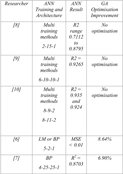
improvement around 8.6% from the non-optimal process. They used ANN to model the different co-substrate including banana stem and optimised it using GA. These works show the application of machine learning in engineering modelling and optimisation have significant impact and improve the production process. Table 1 shows the comparison of biogas production modelling and optimisation using ANN and GA combination.
The objectives of this paper are to present the comparative study of several ANN learning algorithms for process modelling and optimisation and its relation with the optimisation result. In order to achieve these objectives, four types of learning algorithms will be used to model a biogas production process. These prediction models later will be used to find the optimal biogas production using GA optimisation. Previous research had successfully implemented ANN for modelling and GA to find the optimal process yield [6][7]. This paper discusses the impact of different leaning algorithms and how the modelling process can impact on the optimal biogas yield.
2. MATERIALS AND METHODS
2.1. Biogas Datasets
The experiments datasets were taken from study by [11][12] to optimise an anaerobic sequencing batch reactor for biogas production. The experiment was done with 10 litre bioreactor seeded with anaerobic acclimatised banana stem sludge. The input sets are temperature, hydraulic retention time (HRT) and organic loading rate (OLR). Biogas evolved from the reactor was collected and was used as the output value. The experiments used mathematical regression to model the process and used quadratic equation of the response surface methods to optimise the production. The theoretical maximum yield is 1.9497 l/g COD. The factors for the maximum yields are HRT of 11.66 days, OLR of 1.42 gTS/l.d
[image:2.612.314.528.156.458.2]and temperature of 35.8 °C. These results will be compared for results validation.
Table 1. Comparison of biogas modelling and optimisation
2.2. Data Normalisation
Two normalisation categories were used in the experiments to observe the difference of data representation. Binary (0 to 1) normalisation will be used with ANN sigmoid activation and bipolar (-1 to 1) normalisation will be used with hyperbolic tangent activation function. The inputs set and output set were normalised accordingly before the ANN training were done.
2.3. Neural Networks Training
The ANN trainings were utilising Encog 3.2 [13] training algorithms code. Four training algorithms were selected, BP, LM, PSO and Resilient Propagation (RP). BP training algorithms was the easiest training algorithm to train neural networks. It uses gradient descent method of error between the calculated output and the targeted output. While the RP training algorithms is a more modern implementation of BP, it improves the BP training algorithms with each connection has its own delta and change gradually to satisfy the
Researcher ANN
Training and Architecture ANN Result GA Optimisation Improvement
[8] Multi
training methods 2-15-1 R2 range 0.7112 to 0.8795 No optimisation
[9] Multi
training methods 6-10-10-1 R2 = 0.9265 No optimisation
[10] Multi
training methods 8-9-2 8-11-2 R2 = 0.935 and 0.924 No optimisation
[6] LM or BP
5-2-1
MSE < 0.01
8.64%
[7] BP
4-25-25-1
R2 = 0.8703
ISSN: 1992-8645 www.jatit.org E-ISSN: 1817-3195
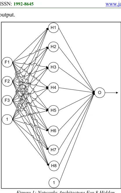
[image:3.612.92.300.75.407.2]287 output.
Figure 1: Networks Architecture For 8 Hidden Neurons
LM training algorithms is a robust training method employing Jacobian matrix. If the Lavenberg’s damping factor is smaller it brings the algorithms close to Gauss-Newton algorithms and if the damping factor is bigger it close to the gradient descent direction. PSO training was applied as a different approach in searching the least error. All the other three algorithms were applying gradient descent or approximation algorithms to minimise the output error. While on the PSO, it has the ability to perform stochastic search of error space. It possesses an alternative concept in finding the least error for the ANN output during the training phase.
The training will be stopped when the weight changes and error were stagnant after 50 epochs. Additional RP training configuration for maximum steps set to 50 and initial update set to 0.1. For PSO, particle counts were set to 20, particles inertia was at 0.72984, cognitive learning rate (C1) was set to 1.49618 and social learning rate (C2) was set to 1.49618.
2.4. Genetic Algorithms Optimisation
The experiments were using Jenetics 1.4.1[14] a Java implementation of genetic algorithms library. The trained networks models from previous tasks were used as the function to be optimised by the GA. Population was set to 50 genomes, with Tournament selection from 5 samples. Roulette Wheel selection was performed to the offspring, while mutation was set to 0.1 and one-point
crossover probability was at 0.1. These
configurations were applied throughout the
experiment to maintain consistency. Further research on pruning the configuration is a research potential to find a better optimise value. For now, these settings were used to obtain the effect of different training algorithms, hidden nodes count and normalisation categories.
3. RESULT AND DISCUSSION
In order to perform the modelling and
optimisation, two main experiments were
conducted. First was to model the process using ANN and afterward the ANN model was optimised by GA. The modelling results are separated to two categories based on the data normalisation methods, binary and bipolar. Two accuracy measurements were used to determine the model performance, the root mean square error (RMSE) and correlation
determination (R2).
3.1 Neural networks modelling
The experiments were using four types of learning algorithms, but only three algorithms were able to produce the modelling result. In most cases of training condition, the traditional BP was failed to produce a usable trained networks. Figure 2 shows the network RMSE for the networks with 1 to 10 hidden neurons using sigmoid activation function. The LM and PSO training were 0.1 RMSE and below on the networks with 3 and more hidden neurons, while networks with 1 and 2 hidden neurons the RMSE is larger. Figure 3 shows
the results measured with data correlation using R2.
Again it shows the R2 for LM is better than PSO
with higher R2 value and the RP training struggled
to produce a better network than LM and PSO. On the hyperbolic tangent activation, the results are better
F1
F2
F3
H1
H2
H3
H4
H5
H6
H7 1
1
O
ISSN: 1992-8645 www.jatit.org E-ISSN: 1817-3195
[image:4.612.71.545.60.588.2]288 Figure 2: RMSE for sigmoid activation
[image:4.612.213.535.71.243.2]Figure 3: R2 for sigmoid activation
[image:4.612.327.546.281.410.2]Figure 4: RMSE for hyperbolic tangent activation
Figure 5: R2 results for hyperbolic tangent activation
Figure 6: Optimisation for sigmoid activation
[image:4.612.329.547.455.586.2]ISSN: 1992-8645 www.jatit.org E-ISSN: 1817-3195
289 Table 2. Weights of input layer
Table 3. Weights of hidden layer
for RP training than on the sigmoid activation. It
was able to model the biogas production with R2
around 0.8, even though the RMSE is only around 0.3. The results suggest that RP is a viable learning algorithm for producing a good model.
Referring to Figure 4 andFigure 5, there are no
significant improvements on LM, but on the PSO training the results of R2 are better than the binary normalisation though the networks RMSE are the same in the region of 0.1. These results show the data representations in normalisation are impacting the correlation to the network output. Larger normalisation range has a better result. Figure 1 shows the example of the networks architecture for ANN modelling using PSO training and hyperbolic tangent activation. It has 8 hidden neurons and the connection weights of the hidden layer from the input layer is shown in Table 2 and Table 3 shows the connection weights from the hidden layer to the output layer.
2.5. Model Optimisation
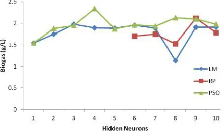
The models were optimised using GA to find the maximum biogas production from the generated ANN models. In Figure 6, the results for
optimisations were not associated directly with the modelling accuracy. These models were trained with sigmoid activation function and the ANN accuracy pattern for LM and PSO were increasing with the addition of hidden neurons to the network. The biogas optimisations for the network models using PSO training were better than the LM training, though the LM models were higher in accuracy.
A selected example of a LM training model with low optimisation yield was a network with 8 hidden neurons and was optimised to a lower production value around 1.13 l/g COD from the 1.85 l/g COD maximum training data production.
This model was trained with RMSE of 0.03 and R2
at 0.99 with epochs at 223. It would be a good candidate for ANN model to predict the biogas production but optimisation was lower than the training data. It may have related to the over fitting condition where the ANN model was trained more than it required. This is the first obstacle the researchers have to aware when using ANN for modelling the engineering process. With accurate model, optimised production or yield was not guaranteed.
Models trained using hyperbolic tangent activation produced better optimisation yield than
the sigmoid function shown in Figure 7. LM and
PSO models were optimised above the maximum targeted production for the networks models with 3 and more hidden neurons using LM training and the networks model with 4 and more hidden neurons using PSO training. The optimised production using PSO training for network with 8 hidden neurons is 2.19 l/g COD, it is an increase of 18.4% improvement in production compared to the training data production.
The highest model optimisation value is 3.85 l/g COD which is more than 100% increase in production. This model was trained with network
RMSE of 0.26 and R2 at 0.851 and it was a good
modelling using the training data. Although the optimised production was high, it is unknown whether the model optimised output can be produced in lab or production line. This is a second complication may occur for model using ANN. Though the model has a very good accuracy and correlation to the training data, the optimisation results produce an enormous biogas yield. It may be used as a solution with assumption of higher production but it is just a false judgement to the theoretical calculations. As ANN is built to replicate human brains, the inside of ANN is
F1 F2 F3 Bias1
H1 -0.54608 0.471107 -0.09204 0.427941 H2 0.974913 0.857733 0.5134 -0.50855 H3 -0.16494 3.179611 0.025061 0.527011 H4 -1.57809 -1.54555 -2.19768 2.079593 H5 0.35234 -1.29639 0.329935 0.66992 H6 11.83694 1.047074 -0.313 0.943739 H7 -0.76787 0.336254 0.183637 0.82394 H8 0.237106 1.998767 1.686089 -1.9847
Output
H1 0.853171
H2 2.36604
H3 10.92567
H4 0.966796
H5 -30.9585
H6 3.234516
H7 -1.67716
H8 0.171346
ISSN: 1992-8645 www.jatit.org E-ISSN: 1817-3195
290 unknown like a black box processing. The calculations or processing to find optimised solution from this model may produce a lower or much higher result because the internal network model not easily explained only the model result or output were evaluated.
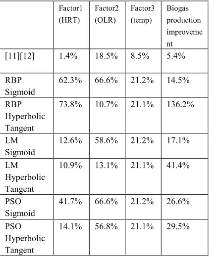
[image:6.612.315.528.252.447.2]Table 4 shows all the maximum biogas production for each training algorithms and compared with the RSM methods results [11][12]. It showed that ANN model better than the mathematical and statistical modelling. The advantages using ANN modelling gives better production output using any algorithms. But the ANN training algorithms produce a very high biogas production which might not reflect the actual process. In Table 5, the ANN modelling by this paper has better output compared to previous study due to implementation of several training algorithms and several network architectures implemented in the experiment. The drawback or limitation of these approach is the knowledge required by the researchers in designing the neural network architectures and applied a proper training algorithms. A knowledge on how a best production model and how its work need to be explored before they applied these methods.
Table 4: Comparison maximum biogas production by each algorithm.
Factor1 (HRT)
Factor2 (OLR)
Factor3 (temp)
Biogas production improveme nt
[11][12] 1.4% 18.5% 8.5% 5.4%
RBP Sigmoid
62.3% 66.6% 21.2% 14.5%
RBP Hyperbolic Tangent
73.8% 10.7% 21.1% 136.2%
LM Sigmoid
12.6% 58.6% 21.2% 17.1%
LM Hyperbolic Tangent
10.9% 13.1% 21.1% 41.4%
PSO Sigmoid
41.7% 66.6% 21.2% 26.6%
PSO Hyperbolic Tangent
14.1% 56.8% 21.1% 29.5%
4. CONCLUSIONS
This paper has presented the relation between modelling accuracy is not directly related to the biogas optimisation results. Model with high accuracy is not guaranteed to produce higher optimised solution. This paper also shows the learning strategies and networks structures (number of hidden nodes) affecting the modelling. A proper network design and training process will generate batter results compared to the mathematical and statistical modelling and optimisation.
Table 5: Comparison with other researchers.
REFERENCES:
[1] E. Betiku, S.O. Ajala, “Modeling and
optimization of Thevetia peruviana (yellow oleander) oil biodiesel synthesis via Musa paradisiacal (plantain) peels as heterogeneous base catalyst: A case of artificial neural network
vs. response surface methodology”, Industrial
Crops and Products, Vol. 53, 2014, pp.
314-322.
[2] X-S. Yang, S. Koziel, and L. Leifsson, “Computational Optimization, Modelling and Simulation: Recent Trends and Challenges”,
Procedia Computer Science, Vol. 18, 2013, pp.
855-860.
[3]. P.E. Chatzistergos, R. Naemi, and N.
Chockalingam, "A method for subject-specific modelling and optimisation of the cushioning properties of insole materials used in diabetic footwear," Medical Engineering & Physics, Vol. 37, No.6, 2015, pp. 531-538
Researcher ANN
Training and Architecture
ANN Result
GA Optimisa
tion Improve
ment
This paper BP, RBP,
LM, PSO
RMSE
0.2 – 0.01
R2
0.4 -0.98
14% - 40%
[6] LM or BP
5-2-1
MSE < 0.01
8.64%
[7] BP
4-25-25-1
R2 = 0.8703
[image:6.612.86.309.453.713.2]ISSN: 1992-8645 www.jatit.org E-ISSN: 1817-3195
291 [4] M. Fischer and X. Jiang, "Numerical
optimisation for model evaluation in
combustion kinetics," Applied Energy, Vol. 156, 2015, pp. 793-803.
[5] I. M. Santos-Dueñas, J. E. J. Hornero, A. M.
Cañete-Rodriguez, and I. Garcia-Garcia,
"Modeling and optimization of acetic acid fermentation: A polynomial-based approach," Biochemical Engineering Journal, Vol. 99, 2015, pp. 35-43.
[6] H. Abu Qdais, K. Bani Hani, and K. Shatnawi.
“Modeling and optimization of biogas
production from a waste digester using artificial
neural network and genetic algorithm”,
Resources Conservation and Recycling, Vol.
54, No. 6, 2010, pp. 359-363.
[7] E.B. Gueguim Kana, J.K. Oloke, A. Lateef, and M.O. Adesiyan, “Modeling and optimization of biogas production on saw dust and other co-substrates using Artificial Neural network and
Genetic Algorithm”, Renewable Energy, Vol.
46, 2012, pp. 276-281.
[8] S.K. Behera, S.K Meher, H-S. Park, “Artificial
neural network model for predicting methane percentage in biogas recovered from a landfill
upon injection of liquid organic waste”, Clean
Technologies and Environmental Policy, 2014,
pp. 1-11.
[9] A. K. Dhussa, S.S. Sambi, S. Kumar, S. Kumar,
S. Kumar, "Nonlinear Autoregressive
Exogenous modeling of a large anaerobic digester producing biogas from cattle waste."
Bioresource Technology, Vol. 170, 2014, pp.
342-349.
[10] K. Yetilmezsoy, F.I. Turkdogan, I. Temizel, A. Gunay, "Development of Ann-Based Models to Predict Biogas and Methane Productions in Anaerobic Treatment of Molasses Wastewater",
International Journal of Green Energy, Vol. 10,
No. 9, 2012, pp. 885-907.
[11] N. Zainol, J. Salihon, R. Abdul-Rahman,
“Kinetic Modeling of Biogas Generation from
Banana Stem Waste” Analysis and Design of
Biological Materials and Structures. Springer
Berlin Heidelberg. Vol. 14, 2012, pp. 175-184. [12] N. Zainol, J. Salihon, R. Abdul-Rahman,
“Biogas production from banana stem waste: optimisation of 10 l sequencing batch reactor”
in IEEE International Conference on
Sustainable Energy Technologies, ICSET, 2008. [13] Encog Machine Learning Framework, 2014,
[Online], Available:
http://www.heatonresearch.com/encog/
[14] Jenetics : Java Genetic Algorithm, 2014,
[Online], Available: