An Algorithm for the Numerical Solution of System of Fractional Differential Equations

(1)

An Algorithm for the Numerical Solution of

System of Fractional Differential Equations

D.Adel Sami Mohamed

Assistance professor

Facutly of science

Raghda Attia Mahmoud

Assistance Lecturer

Higher technological institute for engineering

ABSTRACT

In this paper, we present and discuss an algorithm for the numerical solution of system of the initial value problems of

the form

D



u



f

 

t

,

v

,

D



v



g

 

t

,u

,

u

 

0 

u

₀

,

 

0 v

₀

,

v



0 



,





1 ,

where

D



u

is the derivate of

u of order



,

D



v

is the derivative of v of order



in the sense of Caputo. The algorithm is based on the fractional s s method.

General Terms

Algorithms, numerical solutions, fractional.

Keywords

s method -fractional differential equation - Caputo -fractional derivative.

1. INTRODUCTION

In this we introduce an algorithm for the numerical solution of initial value problems

of the form

 

t

,

v

,

f

u

D





D



v



g

 

t

,u

,

u

 

0 

u

₀

,

 

0 v

0

,

v



0 



,





1 .

(1)

Where

D



u

,

D



v

denote the Caputo fractional differential operators.

Fractional order differential equations are generalizations of classical integer order differential equation These are increasingly used to model problems in the

fluid flow, mechanics, viscoelasticity, biology, physics, engineering and other applications. Brownian motion and fractional diffusion-wave equations and many physical phenomena [1-5].

Most nonlinear fractional differential equations do not have analytic solutions, so approximations and numerical techniques must be used [9-12 ]. The decomposition method [13-18 ] and vartional iteration method [16-18] are relatively new approaches to provide an analytical approximation solution to linear and non linear problems. A comparison between the variational iteration method and Adomian decomposition method for solving fractional differential equations is given in [13]. The fact that the variational iteration method solves non linear equations without using Adomian polynomials can be considered as an advantage of this metho over Adomian decomposition method

.

A few numerical methods for fractional differential equations have been presented in the literature [8-12 ]. In this paper. We begin by introducing some necessary definitions and mathematical preliminaries of the fractional calculus theory which are required for establishing our results. In sections 3 and 4, we introduce the modified trapezoidal rule and a new

derivatives, respectively. In section 5, we derive the fractional s method for the numerical solution of ordinary differential equations. The algorithm itself is presented in details in section 6. In section 7, we present three examples to show the efficiency and the simplicify of the algorithm

.

2. Basic definitions

Definition 2.1

A real function

f

 

x

,

x



0 ,

is said to be in the space

,



C





R

if there exists a real number

p





, such

that

f

 

x



x

p

f

₁

 

x

,

where

f

₁

 

x



C

 

0 ,



,

and it is said to be in the space

C

_m iff

f

 m



C

_,

m



N

.

Definition 2.2

The Riemann-Liouville fractional integral operator of order

,

0 



of a function

f



C

_

,







1 ,

is defined as

 

_{  }

_

_





 





x

t

f

t

dt

x

f

J

0

1

,

1





0 ,

x



0 ,

 

.

0

x

f

x

f

J



Properties of the operator

J

:

For

f



C

_

,







1 ,



,



and







1  

1 J



J



f

 

x



J



f

 

x

 

2 J



J



f

 

x



J



J



f

 

x

 

3

 

_





_

 

















x

J

1

1 Definition 2.3

The fractional derivative of ( ) in the Caputo sense is defined as

 



m

 

x

t



f

 

t

dt

x

f

D

J

x

f

D

x

m m



 







0

1



 



(2)

Definition 2.4

A two-parameter function of the Mittag-Leffer type is defined by the series expansion

 

_

_

,

0 ,

0 .

0

,





_

_















 

k

z

E

Definition 2.5

The Laplace transform of the function f(t) is defined by:

 

_

 

_

_

 

 

0

,

}

;

{

f

t

s

e

f

t

dt

L

s

F

st

Definition 2.6

 









1

, 1

}

{

!

1

  



_

_

k k

k

a

s

at

E

t

k





_

  

   

Lemma 2.7

If

m



1 





m

,

m



N

,

m

C

f



1

,







1 ,

then

 

x

f

 

x

f

J

D

 



(2)

 

_

  

 









1

0

!

0

m

k

k k

k

x

f

x

f

x

f

D

J

 

(3)

3 Results and Theorems

3.1 Modified trapezoidal rule :

We present a review of the modified trapezoidal rule, which is introduced in [20]. This is used to approximate the fractional

integral

J



f

 

t

by a weighted sum of function values at specified points. Suppose that the interval



0 ,

a



is subdivided into k subintervals





1 , j

j t

t of equal width

k a

h by using

the nodes

t_j  jh

, for

j=0,1,……,k .













 







 





 







   

 

2 2

0

1 1

,

, 1



 

a f h f

h

k k

k h

f T

















_

 

_







 















1

1 1

1

2

1

2

1

k

j

t

f

h

j

k

j

k

j

k



  



(4)

is an approximation to the fractional integral

 







  











,

h

E

f

h

f

T

a

t

f

J





_T

,

a



0 ,

0 



. (5)

Furthermore, if

f

 

t



C

2

 

0 ,

a

. There is a constant

C

_

depending only on



so that the error term

E

T



f

,

h

,





(6)

3.2 Generalized Taylor's rule

In this section we introduce a new generalization of Taylor's formula that involves Caputo fractional derivative. This generalization is presented in [20]. We begin by the generalized mean value theorem.

Theorem

(Generalized

mean

value

theorem)

Suppose that f

 

x C

 

0,a and

D



f

 

x



C



0 ,

a



, for 0



1. Then we have

 





_{ }







 

_



D f x

f x

f 

  

 0 1 (7)

with

0 





x

,



x





0 ,

a



.

Proof: in [20].

Theorem :

Suppose that Dn f

 

x , Dn  f

 

x C



a



, 0

1 _

  _,

for 0



1. Then we have





 



   



_{ }











 







  

0 1

1 1

f D n

x

x f D J x f D J

n n

n n n

n

 

  



(8)

where

D

n



D



D





D

 (n-times).

Proof :

The proof can be obtained by using the properties of the Riemann-Liouville fractional integral operator and the Caputo

fractional derivative operator and the relation

:





 



   



_{ }





 







 



D

f

x

J

D

f

x



J

x

f

D

J

x

f

D

J

n n

n

n n n

n

   



  









1 1





 

0 

.



J

n

D

n

f

Theorem: ( Generalized Taylor's rule)

Suppose that Dkf

 

x _C



₀_,a



_for

1 , , 1 ,

0 

 n

k 

, where 01. Then we have





2

 

2

,

h

C

f

a

h

o

h

f

E

T









 

(3)

 

_

_

 



_

_{ }

 



 

_

 

,

1

0

1

0 1 1



  











n i n n i in

x

n

f

D

f

D

i

x

f

  







with

0 





x

,



x





0 ,

a



. (9)

Proof : From (7 ), we have





 



   



_{ }









 



   









n i i in n i i i i i

f

D

i

x

f

D

J

x

f

D

J

0 0 1 1

0

1

    



(10) that is,

 



   



_{ }









 

0 . 1 0 1 1



   _     n i i in n n f D i x x f D J x

f   



(11)

Applying the integral mean value theorem to ( 12 ) yields

   





 



_

 

_



 

_{ }



 

dt

t

x

n

f

D

x

f

D

J

x n

n n n



   

_







0 1 1 1 1

1

   





 





 









  





1 1 1 1       n n x n f D

(12)

3.3 The algorithm for one equation:

In this section we shall derive the fundamental algorithm for the numerical solution of the initial value problem

 

t

f



t

y

 

t



y

D





,

y

 

0 

y

0

,

0 1

.

0 

t

(13)

The new algorithm is based on the modified trapezoidal rule and the fractional Euler's method. Our approach depends on the analytical property that the initial value problem (13 ) is equivalent to the integral equation

 

t

J

f



t

,

y

 

t



y

 

0 .

y







(14)

Let



0 ,

a



be the interval over which we want to find the

approximation thesolution. Suppose that the



0 ,

a



is subdivided into k subintervals



t

_j

,

t

_j_₁



of

equal width

k a

h by using the nodes

t

j



jh

, for

k

j0,1,, . To obtain the solution point



t₁,y

 

t₁



, we substitute

t



t

₁ into (14 ) and we get

 

t₁



J f



t,y

 

t



 

t₁ y

 

0

y    (15)

Now if the modified trapezoidal rule (4 ) is used to approximate



J f



t,y

 

t



 

t₁ with step size

0 1

t

h





, then the resultis

 

_



 

_



_



 

_



 

0

2 ,

0 1 1

0 1

y

t

y

t

f

h

t

y

t

f

h

t

y













  (16)

Notice that the formula on the right-hand side of ( 16 )

involves the term

y

 

t

₁ . So, we use an estimate for

y

 

t

₁ . Fractional Euler's method will suffice for this purpose.

From

 

_

_



,

 



.

1

0 0

0

1

f

t

y

t

h

t

y

t

y











into ( 16 ) yields

 

_



 

_



 

_

_



 







 

0

2 , 1 , 2 , 0 0 0 1 0 0 1 y t y t f h t y t f h t y t f h t y                       

(17)

The process is repeated to generate a sequence of points that

approximate the solution

y

 

t

. The general formula for

our algorithm is:

 

_

_{ }

















 

  









0 ,

1

2

0 0

1

y

t

y

t

f

j

h

t

y

j   





















     _ _ _ _ _     1 1 1 1 1 1 2 1 2 j i i j i j i j

h   



 



t

0

,

y

t

0





f



_





_



 



_



_





 







_



1 1

,

1

1 ,

2

j j

f

t

j

y

t

j

h

t

y

t

f

h



 

3.4 The algorithm for system of two

equations:

In this paper we get a numerical solution of system of fractional differential equations:

 

t

v

f

u

D





,

 

t u f v

D  , ,

u

 

t

₀



u

₀

,

v

 

t

₀



v

₀

1 , 0







(4)

 

_

_{  }













 

  









0 0 0 1

,

1

2 j

j

f

t

v

t

u

t

h

t

u

_j  





 

















 







 

 _ _ _ _ _ _

  



1 1

1

, 1 2

1 2

j

i

i i vt

t f i j i j i

j

h   





_





_



 



_



_





 







_



1 1

,

1

1 ,

2

j j

f

t

j

v

t

j

h

t

v

t

f

h



 

and

 

_

_{ }











 





 

  

  



 

0 0 0 1

, 1

1

2 j j j g t ut vt

h t

v j

 



 



 

















 







 

 _ _ _ _ _ _

  



1 1

1

, 1 2

1 2

j

i

i i ut t g i j i j i

j

h   





_



_

 

_



_





 



_

 1 1, 1

1 ,

2 j j gtj utj

h t

u t g h

 

3.5 Results:

Example

The homogeneous linear system :

v

u

D

.95



 

.

1 

u

₀



.

194 ,

u

v

 

.

1 

v

₀



1 .

17

where

t

₀



.

1

The exact solution

 

1.85 9 ,. 85 . 1 1 .

t

E

t

u



 ,

v

 

t



t

.85

E

₁_.₈₅_,₁_.₈₅

 

t

1.85

from definition (4)

 

_



_

_









0

85 . 85 . 1

85 .

1

85 .

1

k

t

u

,

 



_

_













0

1 . 85 . 1

9 .

85 .

1

k

t

v

Table 1. Numerical values for example with h=.1,

t

₀



.

1

t

Appro

u

_exact

v

_Appro

v

_exact

.2 0.37967 0.27236314 1.429247 1.136372

.3 0.4520032 0.3894135 1.300924 1.132096

.4 0.5786627 0.50580609 1.354413 1.153449

.5 0.7209318 0.62435337 1.425796 1.194041

.6 0.8703125 0.74715702 1.513180 1.251261

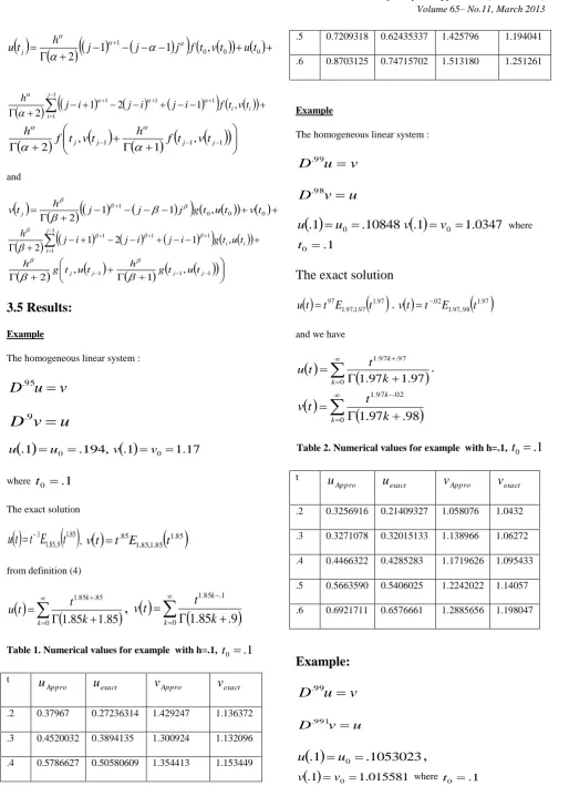
Example

The homogeneous linear system :

v

u

D

.99



u

v

D

.98



 

.

1 

u

₀



.

10848

u

v

 

.

1 

v

₀



1 .

0347

where

1 .

0



t

The exact solution

 

1.97

97 . 1 , 97 . 1 97

t

E

t

u



,

_v

 

_t



_t

.02

_E

₁_.₉₇_,.₉₈

 

_t

1.97

and we have

 

_



_

_









0

97 . 97 . 1

97 .

1

97 .

1

k

t

u

,

 

_



_

_











0

02 . 97 . 1

98 .

97 .

1

k

t

[image:4.595.48.563.45.755.2]

v

t

₀



.

1

t

Appro

u

_exact

v

_Appro

v

_exact

.2 0.3256916 0.21409327 1.058076 1.0432

.3 0.3271078 0.32015133 1.138966 1.06272

.4 0.4466322 0.4285283 1.1719626 1.095433

.5 0.5663590 0.5406025 1.2242022 1.14057

.6 0.6921711 0.6576661 1.2885656 1.198047

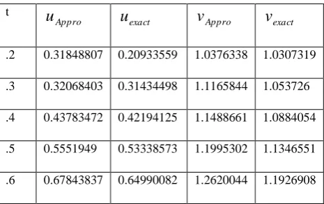
Example:

v

u

D

.99



u

v

D

.991



 

.

1 

u

₀



.

1053023

u

,

 

.1 v₀ 1.015581

v where _t₀ _.₁

u

v

(5)

The exact solution

 

1.981 981 . 1 , 981 . 1 981

t

E

t

u



,

v

 

t



t

.009

E

₁_.₉₈₁_,.₉₉₁

 

t

1.97

then

 

_



_

_









0

981 . 981 . 1

981 .

1

981 .

1

k

t

u

,

 

_



_

_











0

009 . 981 . 1

991 .

981 .

1

k

t

[image:5.595.50.283.256.402.2]

v

t

₀



.

1

t

Appro

u

_exact

v

_Appro

v

_exact

.2 0.31848807 0.20933559 1.0376338 1.0307319

.3 0.32068403 0.31434498 1.1165844 1.053726

.4 0.43783472 0.42194125 1.1488661 1.0884054

.5 0.5551949 0.53338573 1.1995302 1.1346551

.6 0.67843837 0.64990082 1.2620044 1.1926908

4. ACKNOWLEDGMENTS

Our thanks to the experts who have contributed towards development of the template.

5. REFERENCES

[1] P. T. Torvik and R. L. Bagley, On the appearance of the fractional derivative in the behavior of real materials, J. Appl. Mech. 51 (1996), 294-298.

[2] K. B. Oldham, J. Spanier, The Fractional Calculus, Academic Press, New York, 1974.

[3] K. S. Miller and B. Ross, 032An Introduction to the Fractional Calculus and Fractional Differential Equations, John Wiley and Sons, Inc., New York, 1993.

[4] H. Beyer and S. Kemp.e, De.ntion of physically consistent damping laws with fractional derivatives, Z. Angew Math. Mech. 75 (1995), 623-635.

[5] F. Mainardi, Fractional relaxation-oscilation and fractional diffusion-wave phenomena, Chaos, Solitons & Fractals 7 (1996), 1461-1477.

[6] R. Goren.o and F. Mainardi, Fractional calculus: Integral and differential equations of fractional order. In the book Fractals and fractional calculus, (eds.: Carpinteri and Mainardi), New York, 1997.

[7] Y. Luchko and R. Gorne.o, The initial value problem for some fractional differential equations with the Caputo derivative, Fachbreich Mathematicund Informatik, Freic Universitat Berlin, (1998).

[8] I. Podlubny, Fractional differential equations, Academic Press, San Diego,CA, 1999.

[9] K. Diethelm and N. Ford, Analysis of fractional differential equations, J. Math. Anal. Appl. 265 (2002), 229-248.

[10] F. Huang and F. Liu, The time-fractional diffusion equation and fractional advection dispersion equation, ANZIAM J. 46 (2005), 1-14.

[11] R. Goren.o, Fractional calculus: Some numerical methods. In the book Fractals and fractional calculus, (eds.: Carpinteri and Mainardi), New York, 1997.

[12] K. Diethelm, An algorithm for the numerical solution for differential equations of fractional order, Elec. Transact. Numer. Anal. 5 (1997), 1-6.

[14] A. Wazwaz, A new algorithm for calculating Adomian polynomials fo non-linear operators, Appl. Math. Comput. 111 (2000), 53-69.

[15] A. Wazwaz and S. El-Sayed, A new modi.catrion of the Adomian decomposition method for linear and nonlinear operators, Appl. Math. Comput. 122 (2001), 393-405.

[16] N. Shawagfeh, Analytical approximate solutions for nonlinear fractional differential equations, Appl. Math. Comput. 131 (2002), 517-529.

[17] S. Momani, An explicit and numerical solutions of the fractional KdV equation, Math. Comput. Simul. 70(2) (2005), 110-118.

[18] S. Momani, Non-perturbative analytical solutions of the space- and timefractional Burgers equations, Chaos, Solitons & Fractals 28(4) (2006), 930-937.

[19] Z. Odibat and S. Momani, Approximate solutions for boundary value problems of timefractional wave equation, Appl. Math. Comput. 181(1) (2006), 767-774.