Multiple bounded discrete choice contingent valuation: parametric and nonparametric welfare estimation and a comparison to the payment card

(1)

Munich Personal RePEc Archive

Multiple bounded discrete choice

contingent valuation: parametric and

nonparametric welfare estimation and a

comparison to the payment card

Vossler, Christian A.

Department of Economics, University of Tennessee

2003

Online at

https://mpra.ub.uni-muenchen.de/38867/

(2)

MULTIPLE BOUNDED DISCRETE CHOICE CONTINGENT VALUATION: PARAMETRIC AND NONPARAMETRIC WELFARE ESTIMATION AND A

COMPARISON TO THE PAYMENT CARD

Abstract

Inmultiple bounded discrete choice (MBDC) surveys, respondents indicate how

certain they would be to vote in favor of a policy at different prices by choosing, for

example, among “definitely yes”, “probably yes”, “not sure”, “probably no”, and

“definitely no” response options for each price. In estimating non-market values from

MBDC data, past researchers have made markedly different assumptions with respect to

the assumed correlation of within-respondent decisions (one for each price) and the

correspondence of stated payment certainty to actual behavioral intentions. The first

objective of this paper is to provide guidance for future research efforts by

discriminating between existing models and proposing new estimators that relax some

important statistical assumptions of existing models. Contrary to a previous study,

results in this paper suggest that within-respondent decisions should be treated as being

perfectly correlated. The second objective is to examine whether it is worthwhile to

collect the additional information on payment certainty, as it may place additional

cognitive burden on respondents as well as data analysts. Using data from previous

studies, MBDC is compared with the payment card, a related elicitation approach that

does not gauge payment certainty. This comparison provides strong and systematic

evidence that “definitely yes” and “probably yes” MBDC respondents would vote “yes”

(3)

1. Introduction

Over three decades after its introduction, contingent valuation (CV) remains a

popular method for estimating the willingness to pay (WTP) for nonmarket goods,

especially those with a nonuse value component. Accepted practice is to ask a single

dichotomous choice (DC) valuation question, to which respondents simply answer yes

or no as to whether they are willing to pay the offered price for the nonmarket good.

The method is favored on cognitive grounds as answering the valuation question is

similar to voting in an election or making a market purchase. When properly framed,

DC questions also have desirable incentive properties (see Carson, Groves, and

Machina 2000). However, DC is notorious for extracting minimal information on the

respondent’s WTP. Further, researchers caution against assuming respondents are

absolutely certain of their yes or no decision. It is realistic to presume, for example, that

some respondents are indifferent to a yes or no vote (Opaluch and Segerson 1989) and

that subjects have an inherent (and perhaps predictable) randomness in their preferences

(Li and Mattsson 1995).

In order to address concerns about the accepted practice, a laundry list of

alternative elicitation mechanisms have been proposed in attempt to gather more

information on the respondent’s WTP. The double-bounded DC elicitation format and

its variants elicit yes/no answers to a sequence of two or more payment amounts (e.g.,

Cameron and Quiggin 1994). Champ et al. (1997), Johannesson et al. (1999), and

others, ask “yes” DC respondents to indicate how certain they are that they would be

willing to pay the stated price. Other researchers (e.g., Ready, Whitehead, and

Blomquist 1995; Vossler and Kerkvliet 2003) incorporate payment certainty directly

into the valuation question, rather than in a follow-up question. Because of strong

arguments against open-ended questions (see Mitchell and Carson 1987), recent

(4)

The multiple bounded discrete choice (MBDC) format, introduced in the recent

literature by Welsh and Poe (1998), is the only format that asks the respondent about

multiple payment amounts while collecting information on payment certainty.

Specifically, for each price, the respondent indicates how certain she would be to vote

in favor of a policy by choosing, for example, among “definitely yes”, “probably yes”,

“not sure”, “probably no”, and “definitely no” response options. As such, within the

realm of discrete choice valuation formats one can regard the MBDC approach as rather

extreme in terms of the amount of information it attempts to elicit on the respondent’s

WTP.

Since the MBDC approach is still in its infancy, important issues such as

incentive compatibility and bid design effects are not yet fully explored.1 However,

along with the potential wealth of information collected from them, there are good

reasons for considering MBDC questionnaires. First, use of MBDC questionnaires

lessens the burden of optimal bid design endemic to single and double-bounded DC

since they present each respondent with a full range of possible payment amounts

(Alberini 1993; Kanninen 1995). Second, the double-bounded DC elicitation format and

its variants present respondents with (unannounced) follow-up bids based on previous

responses. A wealth of research suggests that anchoring, resentment, or other

unintended response effects force the respondent’s underlying WTP distribution to shift

between initial and follow-up DC valuation questions (Cameron and Quiggin 1994;

Herriges and Shogren 1996; Alberini, Kanninen, and Carson 1997; Bateman et al. 2001;

Whitehead 2002). Bateman et al. (in press) demonstrate that changing the choice set

visible to respondents as they progress along a valuation exercise leads to anomalous

behavior. In contrast, respondents behave consistently with economic theory when the

entire choice set is visible throughout the experiment. Drawing from these results, it is

1

(5)

unlikely that MBDC questionnaires are plagued with unintended response effects as

they present respondents with all payment amounts at the same time.

While there is yet a solid premise for endorsing the MBDC format, given its

potential advantages and the increasing number of field applications that are using this

approach, further investigation is warranted. The main objectives of this paper are to

thoroughly examine the gamut of statistical methods for analyzing MBDC survey data

and to compare the MBDC approach with the payment card (PC), which can be

regarded as a special case of the MBDC questionnaire that does not collect information

on payment certainty. To meet these objectives, this study makes use of data from three

existing studies that use both elicitation formats.

Given the breadth of elicited information, it is not surprising that several

approaches for estimating WTP from MBDC responses already appear in the literature

(Welsh and Poe 1998; Cameron et al. 2002; Alberini, Boyle, and Welsh 2003; Evans,

Flores, and Boyle 2003). However, these analytical methods are somewhat at odds as

important statistical and behavioral assumptions underlying them differ considerably.

While the behavioral intention of the respondent is an open empirical question, the

objective here is to provide guidance as to the appropriateness of underlying statistical

assumptions and to add attractive estimators to the analyst’s choice set.

In an effort to explore the impact of adding a certainty dimension, MBDC is

compared with the PC, which also presents the respondent with a large set of potential

payment amounts, but does not collect information on payment certainty.2 If MBDC

responses can be predictably parceled into yes and no decisions, then the added

complexity of the MBDC approach arguably yields little benefit. Indeed, to the extent

that respondents have cognitive difficulty with the MBDC format, the much simpler PC

may be preferred a priori.

2

(6)

The next section of the paper overviews existing methods for analyzing MBDC

data, and raises important issues with respect to the interpretation and modeling of

responses from this method. Section 3 introduces and provides motivation for

alternative MBDC models. Section 4 briefly describes the data. Statistical assumptions

and model performance is examined in Section 5. Section 6 presents comparisons of

MBDC and PC WTP distributions. Concluding remarks appear in Section 7.

2. Review of Existing Methods for Analyzing MBDC Data

Four models for estimating non-market values from MBDC data appear in the

recent literature: the Welsh-Poe interval model (Welsh and Poe 1998); the Dual

Uncertainty Decision Estimator (DUDE) of Evans, Flores, and Boyle (2003); the binary

choice random effects model (Alberini, Boyle and Welsh 2003); and the ordered choice

model (Cameron et al. 2002; Alberini, Boyle, and Welsh 2003). These models are

distinguishable in terms of (1) the assumed correlation between decisions from the same

individual, and (2) the correspondence between the respondent’s level of payment

certainty and her assumed behavioral intentions.

Welsh and Poe (1998) recode categorical responses into simple yes/no decisions

and model the resulting interval that bounds the respondent’s WTP, employing the

interval data model commonly used for analyzing PC (Cameron and Huppert 1989) and

double-bounded DC (Hanemann, Loomis, and Kanninen 1991) data. Welsh and Poe

(1998) estimate “definitely yes”, “probably yes”, and “not sure” versions of the model.

The name of the model refers to the lowest certainty level recoded as yes. Implicit in

this approach is that one WTP distribution underlies the respondent’s multiple

decisions: i.e., there is perfect response correlation.

Evans, Flores and Boyle (2003) develop the Dual Uncertainty Decision

Estimator (DUDE), which extends the Welsh-Poe interval model by linking categorical

(7)

WTP distribution underlies within-subject responses. However, as an alternative to the

simple yes/no recoding of responses, probability weights are assigned to payment

certainty levels. The Welsh-Poe interval model represents a special case of the DUDE

estimator where recoded yes responses receive a probability weight of 1.0 while no

responses receive a weight of 0.0.

Alberini, Boyle, and Welsh (2003) estimate a binary choice probit model with

random effects. Identical to the Welsh-Poe “probably yes” model, Alberini, Boyle, and

Welsh (2003) treat “definitely yes” and “probably yes” as yes, and other responses as

no. However, rather than using the yes/no responses to define the respondent’s WTP

interval, each yes/no decision becomes a separate observation within a panel data

framework. The multiple observations from the same individual are considered random

draws from separate, but correlated WTP distributions: i.e., responses are freely

correlated. A similar assumption underlies the bivariate probit model used for

double-bounded CV data (Cameron and Quiggin 1994).

Cameron et al. (2002) and Alberini, Boyle, and Welsh (2003) estimate ordered

logit and probit models, respectively.The ordered models treat the certainty categories

as ordered response propensities and, from the data, estimate threshold parameters that

define where respondents switch between certainty levels.3 As in the random effects

probit, an observation is created from each of the respondent’s decisions. However, an

underlying model assumption of Alberini, Boyle, and Welsh (2003) is that each

within-respondent decision is a random draw from an independent WTP distribution – as

though different respondents provided them. Cameron et al. (2002) realize the likely

correlation between within-respondent decisions and, as a compromise, they weight

each observation such that the effective sample size is equal to the number of

respondents.

3

(8)

Table 1 summarizes the underlying assumptions of existing MBDC models. The

log-likelihood functions for these models are included as Appendix A. I now outline the

four research topics explored in this paper using data from three published studies.

Table 1. Overview of Existing MBDC Models

Model (citation)

Correlation of within-respondent decisions

Correspondence between payment certainty

categories and behavioral intentions

Welsh-Poe

(Welsh and Poe 1998)

Perfect correlation Categorical responses recoded as simple yes and no decisions

DUDE

(Evans, Flores, and Boyle 2003)

Perfect correlation Probability weights assigned to categories

Binary choice random effects (Alberini, Boyle, and Welsh 2003)

Responses are freely correlated

Categorical responses recoded as simple yes and no decisions

Ordered choice

(Cameron et al. 2002; Alberini, Boyle, and Welsh 2003)

Responses are independent

Certainty categories treated as ordered choices. Assumed that the

propensity to vote yes switches from negative to positive within the “not sure” category

A. Assumptions regarding within-respondent decisions

MBDC respondents choose among the payment certainty categories for several

possible payment amounts. Existing models assume that these within-respondent

decisions are perfectly correlated, completely independent, or freely correlated (i.e.,

something between independence and perfect correlation). A natural research question

is which assumption is appropriate. Evidence from double-bounded DC questionnaires

(9)

correlated, but can be statistically different due to widely cited response-effects (see

Cameron and Quiggin 1994). It is unclear whether this finding extends to MBDC data,

as respondents see all payment amounts at the same time, rather than in an iterative

manner.

Unlike double-bounded DC, there is no obvious way to test for shifts in the

respondent’s underlying WTP distribution across valuation questions. That is to say, the

price associated with each decision does not vary across respondents and so one cannot

estimate separate WTP functions for each of the respondent’s decisions and then test for

equality of these WTP functions. As an alternative approach, Alberini, Boyle, and Welsh (2003) test whether the correlation coefficient (ρ) in a binary choice random

effects (probit) model is statistically different from zero. Similar to the bivariate probit

model used for double-bounded DC data, the binary choice random effects model

allows within-respondent decisions to be freely correlated and the correlation

coefficient measures the degree of correlation. Failure to reject the hypothesis that the

correlation coefficient is statistically different from zero lends support for treating

within-subject decisions as stemming from independent WTP distributions. Although there is no reliable test of ρ = 1 (see Alberini 1995), a correlation coefficient near 1

provides evidence that within-subject responses can be treated as perfectly correlated.

Alberini, Boyle, and Welsh (2003) estimate the correlation coefficient in a

random effects probit model to be 0.06, which – although statistically different from

zero – suggests that the within-subject response correlation is very small such that

assuming independence is unlikely to significantly distort the standard errors for

estimated model parameters and corresponding WTP estimates. Alberini, Boyle, and

Welsh (2003) appear startled by this result, as they state (footnote 13, p. 50):

(10)

This result carries with it serious implications. First, it would suggest that the

Welsh-Poe and DUDE models are inappropriate. Second, and more importantly, it

would imply that the MBDC approach causes considerable response-effects such as

those that plague responses to follow-up DC questions. If separate WTP functions

underlie each of the respondent’s decisions, then there is little hope that valid WTP

estimates can even be derived from MBDC questionnaires. That is to say, decisions

from the individual are random and correspondingly meaningless. Clearly, the issue of

within-subject response correlation warrants further investigation as it has series

implications for the validity of MBDC surveys.

B. On the use of random effects models

A binary choice random effects model conceptually serves as a compromise

between the interval data models that assume, in essence, a perfect correlation between

within-subject responses, and models that assume response independence. However, the

standard random effects model assumes that the random effect is normally distributed.

Further, the degree of correlation between any two WTP decisions from the same

respondent is assumed to be equal (see Greene 2002, p. 690-693). In general,

distributional assumptions play a key role in the estimation of WTP from discrete

choice cross-section data models. It is therefore likely that estimation of WTP from

discrete choice panel models is sensitive to the assumed distribution of the random

effect. The restriction of equal correlation across within-subject decisions seems

problematic. If the respondent’s underlying WTP distribution does differ across

decisions, it is unlikely that such revisions would occur at an equal rate. For instance,

the respondent may “learn” about their underlying WTP as part of the process of

responding to the valuation questions. The effects of a learning process would

(11)

C. Estimation of WTP from Ordered Choice Models

The use of ordered choice models (e.g., ordered probit, ordered logit, etc.) has

appeal since the analyst can avoid recoding responses into yes or no decisions, or

assigning probability weights to certainty levels.4 In the absence of information on how

certainty category responses reflect actual behavior, a reasonable expectation is for the

switch between a “yes-ish” and a “no-ish” response to occur somewhere within the “not

sure” interval. Unfortunately, unlike in a binary choice model, you cannot tell where the

“propensity to say yes” passes from negative to positive. As such, the model implies a

fitted interval of WTP and not a point estimate (Cameron et al. 2002). Specifically, the

lower WTP bound is where respondents switch between “not sure” and “probably yes”

and the upper bound is where respondents switch between “not sure” and “probably

no”. To obtain mean and median WTP point estimates, Alberini, Boyle, and Welsh

(2003) restrict the two estimated thresholds that bound the “not sure” category to be

symmetric around zero and thus assume that the propensity to say yes passes from

negative to positive at the midpoint of the “not sure” category. An important research

question is whether this symmetry assumption is appropriate. Without making this

assumption a range of possible values has to be considered, and the range of values

tends to be rather wide for useful policy purposes.

D. Insensitivity of WTP estimates to alternative DUDE Model probability assignments

In their Benchmark DUDE Model, Evans, Flores, and Boyle (2003) average

estimates from three psychology studies and derive subjective probability weights of

4

(12)

0.75 and 0.15, respectively to “probably yes” and “probably no” responses.

Probabilities of 1, 0.5, and 0 are assigned to the “definitely yes”, “not sure”, and

“definitely no” categories, respectively. While holding constant the probability weights

for “definitely yes”, “not sure”, and “definitely no” categories, they consider two other

“symmetric” assignments. The Probably DUDE Model assigns weights of 0.6 and 0.4 to

“probably yes” and “probably no” categories, respectively. In the Definitely DUDE

Model, the same categories receive weights of 0.99 and 0.01. Applying these three

DUDE Models to data from the first MBDC field study (Welsh et al. 1995) and

assuming a normal distribution for WTP, they conclude that “within the class of

symmetric (and approximately symmetric) assignments, the parameter estimates from

the DUDE model are relatively insensitive to the specific probability assignment.”

Since the “definitely yes”, “not sure”, and “definitely no” assignments seem defensible,

an interesting research question is whether DUDE models applied to other data show a

similar insensitivity to alternative probability assignments for “probably yes” and

“probably no” categories.

3. New Methods for Analyzing MBDC Data

Indifference Interval Model

The main drawback of the Welsh-Poe and DUDE models is the need to recode

“not sure” responses as either “yes” or “no”, or to assign a probability weight to this

category. Since there is only one study that investigates the criterion validity of MBDC

responses (Vossler et al. 2003b), many researchers may be skeptical about blindly

second-guessing the respondent’s stated intentions. While the ordered choice model

avoids the second guessing of responses, to obtain a WTP point estimate the researcher

has to make some assumption about where in the “not sure” interval the propensity to

say yes passes from negative to positive. However, under the premise that one WTP

(13)

the respondent may be “not sure”. In the studies to date, the majority of respondents do

pick one or more of the three intermediate categories, allowing us to define the

individual’s “not sure” price region with reasonable precision.

Let tL denote the highest price the subject responded at least “probably yes” to

and let tU denote the lowest price the subject responded either “probably no” or

“definitely no” to. Then, the transition between “yes” and “no” falls within the interval

[tL, tU]. The likelihood function is analogous to that of the Welsh-Poe model and is

included in Appendix A.

Nonparametric Estimation of Interval Models

Nonparametric estimators are useful as they are robust against misspecification

of the response probability distribution. Nonparametric estimation seems especially well

suited for MBDC data. Only in rare instances do respondents state a higher level of

payment certainty for a higher payment amount. As a result, the cumulative response

propensities are monotone decreasing with respect to price. This is in contrast to DC

data, where it is common that the raw proportion of yes responses is not monotone (see

Haab and McConnell 1997), and a rule for imposing monotonicity must be used to

construct a valid nonparametric cumulative distribution function (cdf). Given the added

parametric structure of the random effects and ordered choice models, nonparametric

estimation is only feasible for MBDC interval data models, which now includes the

Welsh-Poe, DUDE, and Indifference interval models.

Nonparametric estimation involves three steps: (1) estimating the value of the

WTP cumulative density function (cdf) for each bid amount in the survey; (2) defining

or estimating the upper and lower bounds of the cdf; and (3) a rule for interpolating

between estimated discrete points of the cdf. The value of the WTP cdf at each bid can

be estimated nonparametrically using techniques for survival analysis with censored

(14)

previously applied to single and double-bounded CV data (e.g., Kriström 1990; Carson,

Wilks, and Imber 1994).

Let k =1,…, K denote the order bids are presented in the MBDC survey, Fk

denote the value of the cdf for the kth bid, and tk denote the value of the kth bid. For the

Welsh-Poe and DUDE models likelihood (recall that the Welsh-Poe model is a special

case of the DUDE model), the following log-likelihood is maximized with respect to

F1,…, FK:

{

}

] ln[ )] ( [ ] ln[ )] ( ) ( [ ] 1 ln[ )] ( 1 [

ln ₁ ₁

1 1 1 1 K K i i k k k i i k n i i i n i i i F t WTP P F F t WTP P t WTP P F t WTP P L > = − > − > + − > − = ₋ ₋ = =

∑

_[1]

where the Pi’s are the probability weights in the DUDE model and take on values of 1

or 0 in the Welsh-Poe model. For the Indifference Interval Model the log-likelihood is:

[

]

∑

= − = n i i i UB LB L 1 ln

ln [2]

where LBi = Li0 +

∑

₌

K

k 1 Lik*Fik and UBi =

∑

=

K

k 1 Uik*Fik. Lik equals 1 if bid k is the

highest price respondent i chose either the “definitely yes” or “probably yes” category

for, and equals 0 otherwise; Li0 equals 1 if the respondent gave a “not sure”, “probably

no” or “definitely no” response to the lowest bid, and equals 0 otherwise; and Uik equals

1 if bid k is the lowest price respondent i chose either the “probably no” or “definitely

no” category for, and equals 0 otherwise. Hence, to facilitate estimation, a set of dummy

variables is created to identify the upper and lower bounds of the indifference interval

for each respondent.

The likelihood functions [1] and [2] are straightforward analogs to the

associated parametric models, as presented in Appendix A. In order to construct a valid

(15)

0. As mentioned above, estimates of Fk will be generally non-increasing in price.

Discussion of the case where Fk-1 = Fk for some k is relegated to a footnote.5

After estimating the Fk, one can construct a valid, nonparametric cdf and

calculate mean and median WTP employing the same methods as for nonparametric DC

models. The majority of previous DC applications use the Turnbull lower-bound

estimator (see Haab and McConnell 1997), where the probability mass in each price

interval is massed at the lower end-point of that interval. Rather than adapt this

explicitly conservative approach, as questioned in Poe and Vossler (2002), I follow the

approach of Kriström (1990). For the cdf to be valid, the upper bound (i.e., the highest

price at which F = 0) and the lower bound (i.e., the lowest price for which F = 1) on

WTP need to be chosen or estimated from the data. In the absence of knowledge

regarding the upper bound, linear extrapolation can be used to estimate it:

Upper WTP Bound (tK+1) = 

  

 

− − +

− −

K K

K K K K

F F

t t F t

1

1 _[3]

To preclude negative WTP, one can assume F = 1 at t0 = $0. Alternatively, linear

extrapolation or other methods are available for estimating the lower WTP bound.6

As an estimate of the cdf between bids (including the upper and lower WTP

bound), Kriström uses linear interpolation, which coincides with the assumption that the

probability mass between bids is uniformly distributed and results in a piecewise linear

cdf. With the cdf constructed in this manner, the calculation for Mean WTP is:

5

If Fk-1* = Fk*, a quick solution is to decrease Fk by a negligible amount by decreasing Pi (WTP > tk) by

0.00001 for one respondent. If Fk = 0, then the corresponding bid should be dropped from the model, and

perhaps used as the upper WTP bound. Since no assumption is made regarding the value of the cdf between any two bids, it can be shown that when all individuals respond to all bids, the solution for (1)

has Fk* = 1/n

∑

−

n

i 1

Pi (WTP > tk), and hence if estimation problems are encountered the data can be

easily checked to determine the source of the problem.

6

(16)

Mean WTP = 0.5( )( ₁)

0

1 +

= +

− +

∑

K

k

k k

k t F F

t [4]

where FK+1 = 0 and F0 = 1. Median WTP is the price such that F = 0.5. Since the mean

and median are linear functions of parameter estimates (i.e., the Fk), standard errors and

confidence intervals can be calculated by conventional methods using the maximum

likelihood parameters and covariance matrix. Without assuming normality,

nonparametric bootstrap and simulation techniques are available for generating

confidence intervals (see Poe, Severance-Lossin, and Welsh 1994).

Even if the end goal is to estimate a parametric model, the nonparametric cdf

may be useful in discriminating between parametric distribution functions. For instance,

the nonparametric distribution can be tested against parametric distributions using

standard tests, such as the Smirnov Test (Conover 1980). Further, large differences

between the nonparametric mean and median suggests that an asymmetric parametric

distribution may be appropriate.

Robust Binary and Ordered Choice Models

As discussed in Section 2, estimating a random effects model involves imposing

a rather rigid parametric structure on the data. Alternatively, a robust estimation

approach is available that avoids such structure and is consistent with a random effects

specification under the assumption that within-respondent decisions are freely

correlated. Even if a random effects model is appropriate, a simple cross-section model

that treats all within-respondent decisions as independent observations can be used to

obtain consistent coefficient estimates; however, the estimated covariance matrix is

incorrect (Maddala 1987). White’s (1982) “sandwich” estimator provides a consistent

(17)

(uncorrected) variance matrix from the cross-section model, usually estimated by the

inverse of the Hessian matrix. The sandwich estimator is:

V L ln L

ln n

n V V

K

k

ik n

i K

k

ik

robust _

  

 

 ′

   

 

β ∂ ∂    

 

β ∂ ∂ −

=

∑ ∑

∑

=

=1 =1 1

1 [5]

where lnLikis the value of the (maximized) log-likelihood function for individual i and

bid k. This covariance estimator can be generally applied to discrete choice models. As

such, it serves as a “robust” alternative to both binary and ordered choice random

effects models.

4. Data

In attempt to make general conclusions about the performance of various

modeling approaches, and to corroborate prior findings, this paper analyzes data from

three published studies. To the best of my knowledge, these are the only studies in the

literature that use both MBDC and PC questionnaires. The first dataset (hereafter

referred to as CLASSROOM) comes from a 1994 classroom experiment where students

at Cornell University were asked their annual WTP for reduced fluctuations in Glenn

Canyon Dam releases (Welsh and Poe 1998). The first MBDC field application utilized

an extensive version of this survey (Welsh et al. 1995). Evans, Flores and Boyle (2003)

apply the DUDE model to data from the field application.

The second dataset (POWER, hereafter) comes from a green electricity program

survey conducted in Erie County, New York in 1996. In the survey, Niagara Mohawk

customers were asked how much they were willing to pay per month to join Niagara

Mohawk Power Company’s Green ChoiceTM program, a green electricity program that

would fund a tree planting program and a landfill gas project that could replace fossil

(18)

compared MBDC, PC, open-ended, DC, conjoint analysis, and real purchase decisions.

Cameron et al. (2002) and Poe et al. (2002) provide details on the study. While there

were three MBDC survey versions, the focus in this paper is on the base survey version,

which included bids that correspond closely with the PC survey.

The third dataset (ANGLER, hereafter) is from a survey of anglers who held a

fishing license in Maine during 1994. Anglers were asked to value their fishing

experiences for the 1994 open-water season (April 1, 1994 through September 30,

1994). Specifically, consumer surplus was elicited by asking respondents what they

were willing to pay over and above their total trip expenditures. Split samples were

presented with surveys that presented the array of bids in either ascending (lowest bid

first) or descending (highest bid first) order. Responses from the version with bids in

ascending order are used for comparability with the CLASSROOM and POWER

datasets. Results of the study appear in Alberini, Boyle, and Welsh (2003).

5. MBDC Estimation Results and Model Selection

For parametric models, I adopt the framework of Cameron and James (1987) for

estimating the parameters of a WTP function. Suppose WTP or some transformation of

WTP, f (WTP), is a linear function of covariates Xand a random error term ε such that

i i i X

) WTP (

f = β+ε [6]

where i denotes the individual, βis a vector of parameters to be estimated, and ε has

zero mean, a cumulative distribution function (cdf) denoted by F(ε), and variance σ2.

While WTP is not directly observed through responses to discrete choice questions, the

presence of varying bids, coupled with a choice of F(ε) allow direct estimation of β via

maximum likelihood. Choices of f (WTP) and F(ε) jointly define a distribution for

(19)

In choosing an appropriate parametric distribution for WTP, I compared

estimated normal, log-normal, logistic, log-logistic, and two-parameter Weibull

response functions with corresponding nonparametric estimates under various

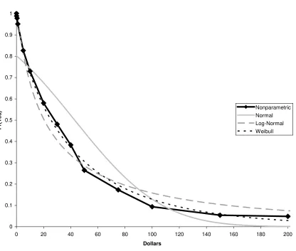
behavioral assumptions. For illustrative purposes, consider Figures 1, 2, and 3, which

display estimated parametric (normal, log-normal, and Weibull) and nonparametric

functions corresponding to the Welsh-Poe “probably yes” model for the three datasets.

In all cases, the normal distribution (the logistic is very similar) noticeably

overestimates the cdf at intermediate bids, and underestimates the cdf for high bids. The

log-normal distribution (the log-logistic is very similar) coincides with the

nonparametric distribution for low to intermediate bids, but overestimates the cdf for

high bids. The Weibull generally approximates the nonparametric cdf well. The

Smirnov Test, which is based on the maximum distance between two cdfs, is used to

test for differences between parametric and nonparametric functions. Using the normal

distribution, the equality of distributions for each of the datasets is rejected at the 5%

significance level. This is somewhat troubling given that in previous analysis of the

datasets, the authors assume either a normal or logistic distribution for ε. The

log-normal is rejected for the POWER dataset only, while the Weibull is never rejected.

Overall, Weibull mean WTP estimates more closely mimic nonparametric estimates

than do estimates from the normal and log-normal distributions. Distribution and

welfare comparisons are qualitatively similar under alternative behavioral assumptions.

Therefore, as a reasonable approximation, all presented parametric models assume a

Weibull distribution. For the Weibull distribution, f (WTP) = ln(WTP) and ε is

distributed extreme value, such that F(ε) = exp[-exp(-ε)].

(20)

0 0.1 0.2 0.3 0.4 0.5 0.6 0.7 0.8 0.9 1

0 20 40 60 80 100 120 140 160 180 200

Dollars

Pr

(Ye

s

) Nonparametric

[image:20.612.122.538.109.462.2]

Normal Log-Normal Weibull

(21)

0 0.1 0.2 0.3 0.4 0.5 0.6 0.7 0.8 0.9 1

0 5 10 15 20 25 30 35 40 45

Dollars

Pr

(Ye

s

) Nonparametric

[image:21.612.118.536.130.532.2]

(22)

0 0.1 0.2 0.3 0.4 0.5 0.6 0.7 0.8 0.9 1

0 200 400 600 800 1000 1200 1400

Dollars

Pr

(Ye

s

) Nonparametric

[image:22.612.120.534.154.535.2]

(23)

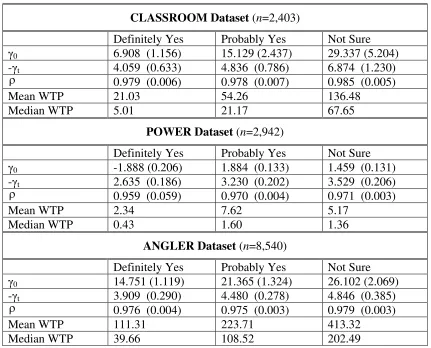
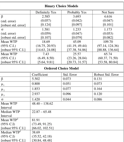
Table 2 presents “definitely yes”, “probably yes”, and “not sure” versions of the

binary choice (Weibull) random effects model for the three datasets. Tables 3a, 4a, and

5a present binary choice models for the same three coding schemes, as well as ordered

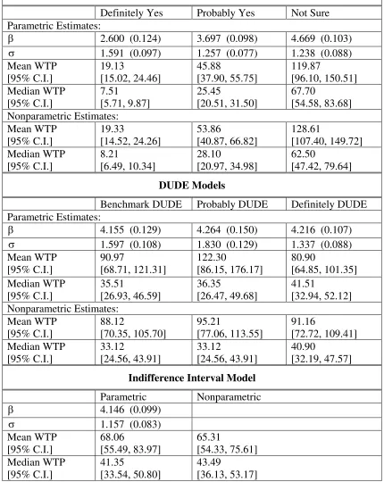
choice models. Tables 3b, 4b, and 5b present parametric and nonparametric interval

models, including: “definitely yes”, “probably yes”, and “not sure” Welsh-Poe models;

Benchmark, Probably, and Definitely DUDE models; and the Indifference Interval

Model.

Random Effects models are estimated using LIMDEP econometric software. For

this model, coefficients correspond with a reparameterization of the WTP function. See

Appendix A for details. All other models are estimated with user-defined maximum

likelihood routines in LIMDEP. Ninety-five percent confidence intervals for mean and

median WTP point estimates are constructed using 10,000 random draws from the

maximum likelihood coefficient vector and covariance matrix, following the approach

of Krinsky and Robb (1986).

A. Examination of Within-Subject Response Correlation

As shown in Table 2, the correlation coefficient ranges from 0.959 to 0.985 in

the various binary choice random effects models. This result is consistent with the

expectation of negligible response-effects stemming from the presence of multiple bids,

but is in stark contrast to Alberini, Boyle, and Welsh (2003), who estimate ρ = 0.06 for

a probit version of the “probably yes” model using the ANGLER dataset. The

difference in estimated correlation coefficients is not due to our omission of covariates

used by Alberini, Boyle, and Welsh (2003), or the choice of parametric distribution. For

completeness, I estimated a probit version of the “probably yes” random effects model –

with and without covariates – and obtained correlation coefficients of 0.947 and 0.985,

respectively. Estimated models are included as Appendix B. SAS and STATA provide

(24)

[image:24.612.109.540.207.555.2]

Table 2. Binary Choice Random Effects Models

CLASSROOM Dataset (n=2,403)

Definitely Yes Probably Yes Not Sure γ0 6.908 (1.156) 15.129 (2.437) 29.337 (5.204)

-γt 4.059 (0.633) 4.836 (0.786) 6.874 (1.230)

ρ _{0.979 (0.006)} _{0.978 (0.007)} _{0.985 (0.005)}

Mean WTP 21.03 54.26 136.48

Median WTP 5.01 21.17 67.65

POWER Dataset (n=2,942)

Definitely Yes Probably Yes Not Sure γ0 -1.888 (0.206) 1.884 (0.133) 1.459 (0.131)

-γt 2.635 (0.186) 3.230 (0.202) 3.529 (0.206)

ρ _{0.959 (0.059)} _{0.970 (0.004)} _{0.971 (0.003)}

Mean WTP 2.34 7.62 5.17

Median WTP 0.43 1.60 1.36

ANGLER Dataset (n=8,540)

Definitely Yes Probably Yes Not Sure γ0 14.751 (1.119) 21.365 (1.324) 26.102 (2.069)

-γt 3.909 (0.290) 4.480 (0.278) 4.846 (0.385)

ρ _{0.976 (0.004)} _{0.975 (0.003)} _{0.979 (0.003)}

Mean WTP 111.31 223.71 413.32

Median WTP 39.66 108.52 202.49

(25)

[image:25.612.114.538.149.633.2]

Table 3a. MBDC Binary and Ordered Choice Models, CLASSROOM Dataset (n=2,403)

Binary Choice Models

Definitely Yes Probably Yes Not Sure

β

(std. error) [robust std. error]

2.585 (0.057) [0.124] 3.693 (0.042) [0.097] 4.616 (0.047) [0.101] σ (std. error) [robust std. error]

1.581 (0.059) [0.107] 1.233 (0.047) [0.079] 1.173 (0.053) [0.082] Mean WTP (95% C.I.) [robust 95% C.I.]

18.69 (16.75, 20.93) [14.63, 24.08] 45.09 (41.19, 49.44) [37.38, 54.86] 109.70 (97.14, 124.36) [88.88, 136.64] Mean WTP (95% C.I.) [robust 95% C.I.]

7.43 (6.49, 8.50) [5.64, 9.81] 25.57 (23.26, 28.04) [20.73, 31.57] 65.74 (60.37, 71.50) [53.58, 80.84]

Ordered Choice Model

Coefficient Std. Error Robust Std. Error

β 5.502 0.073 0.131

1

µ 0.800 0.051 0.073

2

µ 1.853 0.077 0.164

3

µ 2.937 0.096 0.120

σ 1.420 0.044 0.086

Mean WTP Interval

48.40 – 138.62

Median WTP Interval

22.87 – 65.48

Mean WTP1 (95% C.I)

[robust 95% C.I.]

81.91

(73.49, 91.25) [66.02, 102.51] Median WTP1

(95% C.I)

[robust 95% C.I.]

38.69

(35.52, 42.18) [30.84, 48.48]

(26)

[image:26.612.109.539.135.675.2]

Table 3b. MBDC Interval Data Models, CLASSROOM Dataset (n=185)

Welsh-Poe Interval Models

Definitely Yes Probably Yes Not Sure Parametric Estimates:

β 2.600 (0.124) 3.697 (0.098) 4.669 (0.103)

σ 1.591 (0.097) 1.257 (0.077) 1.238 (0.088)

Mean WTP [95% C.I.] 19.13 [15.02, 24.46] 45.88 [37.90, 55.75] 119.87 [96.10, 150.51] Median WTP [95% C.I.] 7.51 [5.71, 9.87] 25.45 [20.51, 31.50] 67.70 [54.58, 83.68] Nonparametric Estimates: Mean WTP [95% C.I.] 19.33 [14.52, 24.26] 53.86 [40.87, 66.82] 128.61 [107.40, 149.72] Median WTP [95% C.I.] 8.21 [6.49, 10.34] 28.10 [20.97, 34.98] 62.50 [47.42, 79.64] DUDE Models

Benchmark DUDE Probably DUDE Definitely DUDE Parametric Estimates:

β 4.155 (0.129) 4.264 (0.150) 4.216 (0.107)

σ 1.597 (0.108) 1.830 (0.129) 1.337 (0.088)

Mean WTP [95% C.I.] 90.97 [68.71, 121.31] 122.30 [86.15, 176.17] 80.90 [64.85, 101.35] Median WTP [95% C.I.] 35.51 [26.93, 46.59] 36.35 [26.47, 49.68] 41.51 [32.94, 52.12] Nonparametric Estimates: Mean WTP [95% C.I.] 88.12 [70.35, 105.70] 95.21 [77.06, 113.55] 91.16 [72.72, 109.41] Median WTP [95% C.I.] 33.12 [24.56, 43.91] 33.12 [24.56, 43.91] 40.90 [32.19, 47.57]

Indifference Interval Model

Parametric Nonparametric

β 4.146 (0.099)

σ 1.157 (0.083)

Mean WTP [95% C.I.] 68.06 [55.49, 83.97] 65.31 [54.33, 75.61] Median WTP [95% C.I.] 41.35 [33.54, 50.80] 43.49 [36.13, 53.17]

(27)

[image:27.612.109.539.141.623.2]

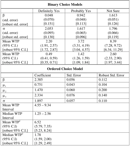
Table 4a. MBDC Binary and Ordered Choice Models, POWER Dataset (n=2,942)

β

0.49 (0.41, 0.59) [0.35, 0.71] 1.42 (1.26, 1.59) [1.09, 1.84] 2.60 (2.33, 2.90) [1.97, 3.44]

β 2.385 0.056 0.112

1

µ 0.751 0.043 0.104

2

µ 1.470 0.060 0.200

3

µ 2.334 0.076 0.140

σ 1.897 0.057 0.110

Mean WTP Interval

4.55 – 9.34

Median WTP Interval

1.25 – 2.56

Mean WTP1 (95% C.I)

[robust 95% C.I.]

6.52

(5.79, 7.35) [5.23, 8.24] Median WTP1

(95% C.I)

[robust 95% C.I.]

1.78

(1.59, 2.00) [1.29, 2.49]

(28)

[image:28.612.110.538.89.662.2]

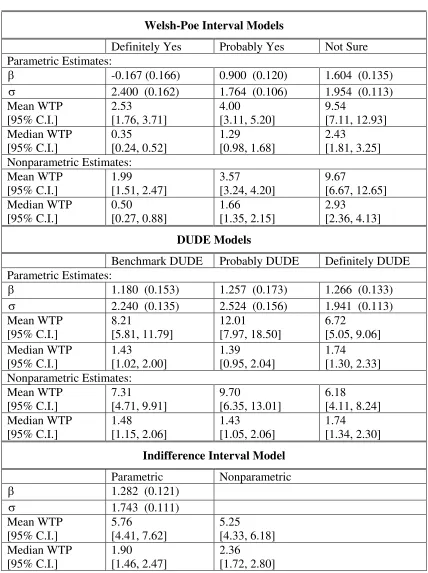
Table 4b. MBDC Interval Data Models, POWER Dataset (n=260)

Welsh-Poe Interval Models

β -0.167 (0.166) 0.900 (0.120) 1.604 (0.135)

σ 2.400 (0.162) 1.764 (0.106) 1.954 (0.113)

Mean WTP [95% C.I.] 2.53 [1.76, 3.71] 4.00 [3.11, 5.20] 9.54 [7.11, 12.93] Median WTP [95% C.I.] 0.35 [0.24, 0.52] 1.29 [0.98, 1.68] 2.43 [1.81, 3.25] Nonparametric Estimates: Mean WTP [95% C.I.] 1.99 [1.51, 2.47] 3.57 [3.24, 4.20] 9.67 [6.67, 12.65] Median WTP [95% C.I.] 0.50 [0.27, 0.88] 1.66 [1.35, 2.15] 2.93 [2.36, 4.13] DUDE Models

Benchmark DUDE Probably DUDE Definitely DUDE Parametric Estimates:

β 1.180 (0.153) 1.257 (0.173) 1.266 (0.133)

σ 2.240 (0.135) 2.524 (0.156) 1.941 (0.113)

β 1.282 (0.121)

σ 1.743 (0.111)

(29)

[image:29.612.109.541.161.651.2]

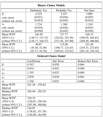
Table 5a. MBDC Binary and Ordered Choice Models, ANGLER Dataset (n=8,540)

β

48.87 (45.46, 52.49) [43.71, 54.78] 115.08 (108.77, 121.63) [105.62, 125.61] 221.40 (210.31, 232.85) [201.24, 244.10]

β 6.542 0.030 0.064

1

µ 0.674 0.023 0.040

2

µ 1.355 0.032 0.089

3

µ 2.078 0.038 0.063

σ 1.520 0.023 0.046

Mean WTP Interval

241.28 – 476.82

Median WTP Interval

102.49 – 202.55

Mean WTP1 (95% C.I)

[robust 95% C.I.]

339.19

(320.87, 358.34) [297.80, 388.06] Median WTP1

(95% C.I)

[robust 95% C.I.]

144.05

(136.82, 151.78) [126.88, 164.09]

(30)

[image:30.612.111.541.86.659.2]

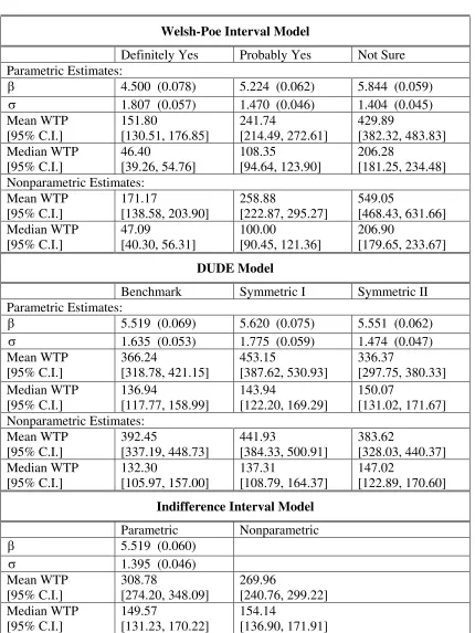
Table 5b. MBDC Interval Data Models, ANGLER Dataset (n=622)

Welsh-Poe Interval Model

β 4.500 (0.078) 5.224 (0.062) 5.844 (0.059)

σ 1.807 (0.057) 1.470 (0.046) 1.404 (0.045)

Mean WTP [95% C.I.] 151.80 [130.51, 176.85] 241.74 [214.49, 272.61] 429.89 [382.32, 483.83] Median WTP [95% C.I.] 46.40 [39.26, 54.76] 108.35 [94.64, 123.90] 206.28 [181.25, 234.48] Nonparametric Estimates: Mean WTP [95% C.I.] 171.17 [138.58, 203.90] 258.88 [222.87, 295.27] 549.05 [468.43, 631.66] Median WTP [95% C.I.] 47.09 [40.30, 56.31] 100.00 [90.45, 121.36] 206.90 [179.65, 233.67] DUDE Model

Benchmark Symmetric I Symmetric II Parametric Estimates:

β 5.519 (0.069) 5.620 (0.075) 5.551 (0.062)

σ 1.635 (0.053) 1.775 (0.059) 1.474 (0.047)

β 5.519 (0.060)

σ 1.395 (0.046)

(31)

Given the very large and statistically significant correlation coefficients, models

estimated under the premise of within-subject response independence are inappropriate.

However, coefficient estimates from ordered or binary choice models where the

responses are pooled but the correlation structure is ignored are consistent (Maddala

1987), and so the concern lies in the estimated standard errors. Tables 3a, 4a, and 5a

report binary and ordered choice model coefficients and WTP estimates. Two sets of

coefficient standard errors and corresponding 95% confidence intervals for WTP are

reported. The first set assumes within-subject independence while the “robust”

estimates are calculated using the “sandwich” estimator, which takes account of

within-subject response correlation. In all cases, robust standard errors and 95% confidence

intervals are noticeably larger, implying that inferences based on uncorrected standard

errors are problematic. For the binary choice models using the CLASSROOM dataset,

for example, the robust standard errors are approximately twice as large as the

uncorrected errors.

B. Monte Carlo and Empirical Evidence on Model Performance

It is clear that that the independence assumption is inappropriate, although the

correlation coefficient estimates do not serve in and of themselves as a basis for

choosing between random effects and interval data models. The correlation coefficients

are very close to 1, but there is no reliable test of ρ= 1 (Alberini 1995). Even if there

were such a test, concerns over distributional and other assumptions imposed in the

random effects model call into question its usefulness.

As an alternative mode of investigation, simple Monte Carlo experiments were

conducted to gain insight into the relative performance of random effects versus interval

data models for analyzing MBDC data under the premise of perfect correlation of

within-respondent decisions. Another feasible alternative is to estimate a binary choice

(32)

well. The experiment is set up as follows. Numbers representing underlying WTP

amounts for a sample of 100 individuals are randomly drawn from the normal

distribution. For each individual a set of yes/no indicator variables are constructed by

comparing the individual’s WTP to a set of payment thresholds. Specifically, the set of bids is {0,5,10,15,20,25,30,35,40,45,50,55,60}, there are no response errors, and ρ = 1:

a yes response is recorded if WTP > bid and otherwise a no response is recorded.7

There are 13 bids and so this procedure produces 1,300 total observations. These

observations are used to estimate mean WTP from binary probit and random effects

probit models. The upper and lower WTP bounds for each individual are created by

identifying the two consecutive survey bids that bound the individuals’ WTP.8 An

interval data model estimates mean WTP using the set of WTP bounds for the 100

individuals.

Table 6 presents results from two Monte Carlo experiments. In the first

experiment, individual WTP values drawn from a normal distribution with a mean of

$30 and standard deviation of $30. In the second experiment, the mean is $50 with a

standard deviation of $30. Note that the expected mean WTP in experiment 1 is in the

center of the bid distribution, while the mean and standard deviation of WTP in

experiment 2 is such that many respondents have WTP amounts larger than the highest

bid. This is analogous to a situation of a survey with a poor bid design. There are 500

replications in each experiment.

Several interesting results stem from the experiments. First, the correlation

coefficients average 0.972 and 0.973, respectively, in the two experiments and the range

of values across replications is small (0.960 to 0.984). Second, the mean-squared error

(MSE) is approximately ten times larger for the random effects probit versus the other

7 _{Other experiments were run where the respondent’s WTP is highly correlated across bids (ρ=0.95).}

There was no real difference in results, except for slightly lower random effect probit estimates of ρ.

8

As standard in interval models, the lower bound is -∞ if WTP is less than the smallest bid and the upper

(33)

two models. In a Monte Carlo comparison between the interval model and a bivariate

probit for estimating WTP from double-bounded CV data, Alberini (1995) finds that the

latter model is inferior in terms of MSE. Third, in Experiment 2, where the bid design is

relatively poor, WTP from the random effects probit is 6% below the true value on

average and is off by as much as $13.90 (28%) in individual trials. In contrast, both the

interval model and binary probit perform well in terms of accurately estimating mean

WTP, with no evidence of systematic bias. The MSE of the interval model is

approximately 20% smaller than the binary probit, but this is to be expected. Overall, it

appears that the interval model is preferred under the premise that within-respondent

[image:33.612.112.540.393.697.2]

decisions are highly correlated.

Table 6. Monte Carlo Results: Performance of the Probit, Random Effect Probit, and Interval Models

Experiment 1: Mean (β) = $30, ρ = 1 (100 individuals, 500 Replications)

Probit Random Effects

Probit

Interval Model

Mean WTP MSE maxβˆ −β

30.07 0.78 3.19

30.43 11.01 9.90

30.07 0.65 2.55 ρ

Std. dev. Range

0.000 0.972

0.003

0.962 – 0.984

1.000

Experiment 2: Mean (β)= $50, ρ = 1 (100 individuals, 500 Replications)

Probit Random Effects

Probit Mean WTP

MSE maxβˆ −β

50.20 2.66 5.58

47.23 22.35 13.90

50.22 2.05 4.66 ρ

Std. dev. Range

0.000 0.973

0.004

0.960 – 0.983

(34)

Results from the Monte Carlo experiments do carry over to actual MBDC WTP

estimates. Both the average (0.975) and range of coefficient values (0.959 to 0.985)

estimated with actual MBDC data are strikingly close to the simulated values. While not

a proof, this suggests that actual within-respondent decisions for the three datasets could

be perfectly correlated. Quite generally, coefficient and WTP estimates are very similar

between the binary choice and comparable Welsh-Poe interval models. Random effects

model estimates are in the ballpark of those from comparable models but differ

noticeably in instances. For the POWER dataset, estimated mean and median WTP is

actually larger in the “probably yes” than in the “not sure” model, where more

responses are treated as “yes”. Actual estimation results coupled with the relatively

large MSE observed in Monte Carlo experiments serve to illustrate the routine’s

apparent difficulty in accurately identifying WTP.

C. Comparison of WTP from Ordered Choice and Indifference Interval Models

Both the ordered choice model and the Indifference Interval model can estimate

WTP without the need to recode or second-guess categorical responses. As discussed in

Section 2, to estimate WTP from the ordered choice model the analyst must make the

untestable assumption that the fitted WTP interval corresponding to the “not sure”

category is symmetric. Such an assumption is not necessary for the Indifference Interval

model. The key difference between modeling approaches is that the Indifference

Interval estimator directly models the individual’s “not sure” price interval while the

ordered choice model attempts to estimate the “not sure” interval from the data.

Maintaining the hypothesis that a single underlying WTP distribution drives all

within-respondent decisions, the Indifference Interval Model is presumably the preferable

approach. Therefore, testing for equality of WTP between ordered choice and

Indifference Interval models sheds light on whether the symmetry assumption is

(35)

version of the ordered choice model and the indifference model. Since I use simulation

methods to derive the distributions for our WTP point estimates, the method of

convolutions (Poe, Severance-Lossin, and Welsh 1994) is appropriate for testing

between two WTP point estimates. Both mean (CLASSROOM: pc = 0.230; POWER: pp

= 0.503; ANGLER: pa = 0.250) and median (pc = 0.677; pp = 0.783; pa= 0.336) WTP

estimates are not statistically different at the 5% level for all datasets. As such, this

lends qualified support of the “symmetry” restriction needed to identify WTP point

estimates in the robust ordered model. It is likely that in some applications, the

individual’s “indifference interval” is not well defined. This can happen when many

respondents are not willing to pay the first bid amount or otherwise do not choose the

intermediate categories over the range of prices. In such situations, the robust ordered

choice model is preferable.

D. Replication of Evans, Flores, and Boyle

Evans, Flores, and Boyle (2003) find that welfare estimates are insensitive to the

different probability assignments of the Benchmark, Probably, and Definitely DUDE

models. Using the method of convolutions, I conduct pair-wise tests of equality between

mean or median WTP estimates from the different parametric specifications. Using the

method of convolutions, I find that Probably DUDE and Definitely DUDE mean WTP

estimates are statistically different at the 5% significance level for all datasets (pc =

0.050; pp = 0.026; pa = 0.004). However, median WTP is never statistically different

between these same models. In all possible cases, mean and median WTP estimates

from the Benchmark DUDE model are not statistically different than estimates from the

Probably and Definitely DUDE models. Overall, median WTP estimates are insensitive

to alternative “probably yes” and “probably no” DUDE model probability assignments.

However, when the goal is to estimate mean WTP, these same probability assignments

(36)

6. Comparing MBDC with the PC

The MBDC elicitation mechanism can be regarded as a PC with payment

certainty as an added dimension. In this section, I examine how respondents behave in

the absence of the payment certainty categories.9 This exploration is deliberately

comprehensive as I consider a multitude of different MBDC models – each with

differing behavioral assumptions, compare both WTP point estimates and estimated

WTP functions, and employ both parametric and nonparametric approaches.

To limit the scope of comparisons, the focus is on the various interval data

models as well as the robust ordered choice model. Note that binary choice models

mimic the Welsh-Poe models. The (parametric) random effects models are ignored for

obvious reasons. PC data are analyzed using the parametric and nonparametric versions

of the interval data model.10 Comparisons are made between estimated nonparametric

and various parametric distributions for the PC data, analogous to those described for

MBDC data in Section 4. Again, I find that the Weibull distribution serves as a

reasonable approximation for the underlying WTP distribution.

Table 7 presents estimated Weibull and nonparametric PC interval models. I

first test for equality between PC and various MBDC parametric WTP functions, using

the likelihood ratio test:

LR = −2

[

lnL₁₌₂ −(lnL₁+lnL₂)

]

~ χ2 (r) [7]

where lnL1 and lnL2 are values of the log-likelihood at solution for the independent PC

and MBDC models, lnL1=2is the value of the log-likelihood for a model that pools both

datasets and estimates a common parameter vector (β,σ), and r is the number of

restrictions. Since the sample sizes differ between corresponding PC and MBDC

9

Despite several requests, our efforts to acquire the PC data from the ANGLER study were unsuccessful.

10

(37)

samples in the POWER dataset, I use sampling weights such that each sample, rather

than each observation, receives equal weight. The relative error variances are allowed to

differ by data type, as any difference in error variance between data type would distort

estimated parameters of a pooled model. When pooling the ordered choice and PC data,

no symmetry restriction is needed as the PC data allow us to identify all four ordered

[image:37.612.112.537.265.504.2]

thresholds (i.e., the normalization µ₀= 0 is not imposed; see Cameron 2002).

Table 7. Payment Card Models

Parametric Models

CLASSROOM Data POWER Data

β 3.635 (0.096) 0.938 (0.098)

σ _{1.241 (0.074)} _{1.548 (0.082)}

Mean WTP [95% C.I.]

42.71

[35.52, 51.54]

3.51

[2.92, 4.24] Median WTP

[95% C.I.]

24.05

[19.46, 29.66]

1.45

[1.16, 1.81] Nonparametric Models

CLASSROOM Data POWER Data

Mean WTP [95% C.I.]

43.84

[35.65, 52.01]

3.57

[2.87, 4.27] Median WTP

[95% C.I.]

21.58

[17.53, 28.35]

1.36

[1.22, 1.94]

n 188 292

Notes: Standard errors are in parentheses. All estimated parameters are statistically different from zero at the 5% level. The two-parameter Weibull distribution is assumed for parametric models.

Employing a 5% significance level, I fail to reject the hypothesis of equal WTP

functions only when comparing PC and “probably yes” Welsh-Poe interval models [CLASSROOM: χc2(2)=0.205, pc = 0.902; POWER: χp2(2) = 0.060, pc = 0.970]. While

comparisons of welfare estimates are not as clean, I fail to reject both equal mean and

median WTP between PC and “probably yes” models only [means: pc = 0.599, pp =

0.423; medians: pc = 0.713, pp = 0.519]. For the POWER dataset, there are several

(38)

the results of LR tests and mean WTP tests, this result is merely coincidental as

underlying response functions fundamentally differ.

To explore the robustness of the findings, the Smirnov Test is used to compare

estimated nonparametric distribution functions.11 Paralleling results for the LR tests, I

fail to reject the hypothesis of equal WTP distributions between PC and “probably yes”

models only and this result holds across datasets. The maximum distances between

these WTP distributions are 6.6% and 8.4%, respectively, for the CLASSROOM and

POWER datasets. Tests of WTP point estimates likewise coincide with the results from

parametric tests, as I only fail to reject equality between PC and “probably yes” MBDC

models for both point estimates.

Overall the evidence is clear – in the absence of the certainty response

categories, otherwise “definitely yes” and “probably yes” respondents will vote yes,

while “not sure”, “probably no”, and “definitely no” respondents will vote no. While

presumption may be that some “not sure” respondents would vote yes and others vote

no, neither the Indifference Interval, ordered choice model, nor any of the DUDE

models match PC response functions or both mean and median WTP estimates.

So, what are the implications of this finding? It does suggest that, when not

given the option, “not sure” respondents tend to vote “no”. This coincides closely with

findings from CV survey comparisons with actual voting behavior (Carson, Hanemann,

and Mitchell 1986; Champ and Brown 1997; Vossler et al. 2003a) and evidence from

pre-election polls (Magelby 1989), where voters who are undecided before an election

overwhelmingly vote “no” on Election Day. If we may extrapolate from these findings,

it may be the case that “not sure” responses are an indication that the respondent would

11

(39)

not actually pay the corresponding amount if faced with an analogous real purchase

situation.

In the lone MBDC field validity test (Vossler et al. 2003b), from which the

POWER data comes from, MBDC responses correspond with actual purchase decisions

only when the vast majority of “definitely yes” and “probably yes” responses are treated

as yes, and other responses are treated as no. Consistent with our findings, PC decisions

match actual purchase behavior. If this finding is consistent in future validity studies,

this suggests that virtually nothing is gained by inclusion of the payment certainty

categories. Similarly, PCs are preferred as they reduce the cognitive burden of

respondents as well as data analysts. Clearly, the issue of whether “not sure” responses

reflect actual or fictional uncertainty introduced by the inclusion of such a response

option in a contingent market survey warrants further research.

7. Concluding Remarks

In multiple bounded discrete choice (MBDC) surveys, respondents face multiple

payment amounts for a nonmarket good and indicate their level of payment certainty for

each amount. As it stands, this elicitation mechanism attempts to gather much more

information on the respondent’s WTP than standard DC questions. Making use of three

existing datasets, I explore the issue of data analysis and compare MBDC with the

payment card (PC), which presents the respondent with multiple payment amounts but

does not collect information on payment certainty.

Given the nature of the data, two important issues to consider when analyzing

MBDC responses are how to treat the multiple responses from the same individual and

how payment certainty levels correspond with real behavioral intentions. Contrary to

past research, there is compelling evidence in favor of treating the within-respondent

decisions as perfectly correlated, thus driven by a single underlying WTP distribution.

(40)

0.959 to 0.985 using random effects models. Further, empirical WTP estimates and

evidence from Monte Carlo experiments provide support for favoring interval models,

which assume perfect correlation, over random effects models in terms of their ability to

estimate WTP accurately. Thus, overall this study provides strong guidance for model

selection. The set of existing analytic approaches is expanded by introducing

nonparametric interval model estimators, an Indifference Interval model which serves

as a alternative to the ordered choice model used in past research, and a procedure for

correcting the covariance matrix from models that assume within-subject response

independence, so that valid inferences may be drawn from such models.

Comparisons between PC and various MBDC models, which differ largely in

terms of how payment certainty responses are treated, reveal a strong compatibility

between PC and MBDC models that treat “definitely yes” and “probably yes” responses

as yes and all other responses as no. In fact, this finding is consistent across datasets and

holds for both parametric and nonparametric response functions as well as mean and

median WTP estimates. For all other MBDC models, both parametric and

nonparametric response functions are statistically different from corresponding PC

functions. In the lone field validity test of MBDC surveys (Vossler et al. 2003b), this

same recoding of certainty responses into yes/no decisions is needed for correspondence

between survey responses and revealed behavior. Evidence from CV survey responses

and actual voting behavior, as well as pre-election polls suggests likewise that the

majority of “undecided” pre-election respondents vote no in actual elections. Evidence

from field research, coupled with comparisons between PC and MBDC responses,

suggests that all relevant information from the respondent is attainable through PC

surveys. That is to say, the inclusion of the payment certainty categories may be

unnecessary and simply serve to add complication for the respondent as well as the data