Head First Linearization with Tree Structured Representation

279

Head-First Linearization with Tree-Structured Representation

Xiang Yu, Agnieszka Falenska, Ngoc Thang Vu, Jonas Kuhn Institut f¨ur Maschinelle Sprachverarbeitung

Universit¨at Stuttgart, Germany

[email protected]

Abstract

We present a dependency tree linearization model with two novel components: (1) a tree-structured encoder based on bidirectional Tree-LSTM that propagates information first bottom-up then top-down, which allows each token to access information from the entire tree; and (2) a linguistically motivated head-first decoder that emphasizes the central role of the head and linearizes the subtree by in-crementally attaching the dependents on both sides of the head. With the new encoder and decoder, we reach state-of-the-art performance on the Surface Realization Shared Task 2018 dataset, outperforming not only the shared tasks participants, but also previous state-of-the-art systems (Bohnet et al., 2011; Pudup-pully et al.,2016). Furthermore, we analyze the power of the tree-structured encoder with a probing task and show that it is able to recog-nize the topological relation between any pair of tokens in a tree.

1 Introduction

Surface realization is a natural language genera-tion task that searches for the natural linear order of words given an unordered syntax tree. Often, the task is accompanied by predicting word inflec-tion, as in two previous surface realization shared tasks (Belz et al., 2011, 2018). As morphologi-cal inflection prediction is in itself a separate task (Cotterell et al.,2016), we mainly focus on the lin-earization in this paper.

Syntactic linearization has been extensively studied in the literature. Earlier work mostly fo-cuses on grammar-based approaches using dif-ferent syntactic formalisms (Elhadad and Robin,

1992;Lavoie and Rainbow, 1997; Carroll et al.,

1999). Recently, with the increasing availability of annotated treebanks, statistical methods gain pop-ularity (Langkilde and Knight, 1998; Bangalore and Rambow,2000;Filippova and Strube,2009).

Among the most successful statistical lineariza-tion systems, Bohnet et al. (2010) employ the divide-and-conquer strategy and use beam search to incrementally find the best linearization for each subtree; Liu et al. (2015) propose a transi-tion system akin to dependency parsing that pro-duces a sentence that respects the given tree con-straints, which is later improved by Puduppully et al.(2016) with look-ahead features. Both ap-proaches rely on rich feature templates to cap-ture the structural information from the input and score the (partial) output sequence, and use the perceptron to learn the parameters. Both lineariz-ers achieve state-of-the-art performance on the Surface Realization Shared Task 2011 data (Belz et al.,2011) as part of a pipeline or joint system for the full task including deep semantic generation and word inflection (Bohnet et al., 2011; Pudup-pully et al., 2017). However, to the best of our knowledge, the two linearizers alone have never been directly compared. Also, they have not been tested on the data from the recent shared task (Belz et al.,2018), where they could have served as very strong baselines to put recent developments into context.

Song et al. (2018) are the first to use a neu-ral model for syntactic linearization; they adapt the neural dependency parsing model by Chen and Manning(2014) to predict transitions for lin-earization, which essentially replaces the percep-tron with an MLP for the transition system inLiu et al. (2015). However, their adoption of neural models only takes advantage of the token-level representation such as word embeddings, while the structural information is still not well modeled. Recently, many neural models are proposed to represent graph structures, cf. Zhou et al.(2018) for an overview. Among them, Tree-LSTM, in particular the Child-Sum variation (Tai et al.,

dependency trees. It differs from the sequen-tial LSTM (Hochreiter and Schmidhuber, 1997) in that it aggregates the hidden states of multi-ple dependents by summation. It is in turn im-proved by adding the attention mechanism to the hidden states (Zhou et al.,2016), so that each de-pendent influences the head representation to dif-ferent degrees.Miwa and Bansal(2016) propose a bidirectional extension that traverses the tree both bottom-up and top-down to allow the tokens ac-cess information from their descendants as well as ancestors. We adopt and combine their proposed models to represent the tree structure in our task, while improving the bidirectional extension by us-ing the output of the bottom-up pass as the input for the top-down pass, so that each token can ac-cess information from all other tokens.

In most linearization models, the incremental generation algorithm follows the left-to-right se-quential order. However, in the linguistic study, the head position often plays a central role in de-scribing the constraints and optimization of word orders (Gibson, 1998; Liu, 2010; Futrell et al.,

2015). In the linearization models that employ left-to-right generation, such word order proper-ties are only implicitly reflected in the features, if at all. Inspired by the above-mentioned study on head-oriented word order constraints, we adopt an improved linearization algorithm, in which we generate the sequence starting from the head and expanding to both directions. The head-first gener-ation order can easily capture the constraints, since it naturally separates the decision into two aspects: (1) which side of the head to append the depen-dent and (2) which dependepen-dent to attach closer to the head, which exactly correspond to the two as-pects of the word order constraints, namely (1) the direction of the dependent and (2) the distance of dependent to the head. The algorithm is some-what similar to He et al. (2009), which also em-phasizes the central role of the head by first pre-dicting for each dependent which side of the head it is placed. However, they exhaustively score all permutations, which could be intractable for sub-trees with too many dependents, while we use in-cremental beam-search to guarantee the efficiency.

In this context, our contribution in this work is threefold: (1) we incorporate the tree-based repre-sentation to the linearization models; (2) we im-prove the linearization algorithm with plausible linguistic intuition; and (3) we conduct a

compre-cheio

tesouro

este de

estar .

estar cheio de este tesouro .

est´a cheia de estes tesouros .

est´a cheia destes tesouros. (1) linearization

(2) inflection

(3) detokenization

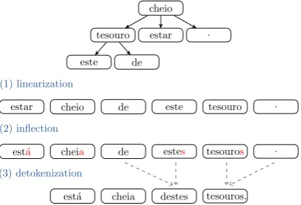
Figure 1: Overview of the pipeline and an example of the process from an unordered dependency tree to the final sentence.

hensive comparison with several strong baselines on the recent multilingual linearization shared task data, and achieve state-of-the-art performance.

2 Model

We use a pipeline system for the surface realiza-tion task, consisting of three steps: linearizarealiza-tion (§2.1), inflection (§2.2), and detokenization (§2.3). Figure1gives an overview of the pipeline along with an example from the input tree to output text. The input is an unordered dependency tree. We first linearize the tree to obtain an ordered se-quence of tokens; then inflect each lemma into the corresponding word form given the morphologi-cal information; and finally contract some words into one token and remove the empty space around some punctuation marks, obtaining the output Por-tuguese text “est´a cheia destes tesouros.” (it is full of these treasures).

To encode the tokens with tree-structured in-formation, we use a bidirectional attentive Tree-LSTM model improved upon previous work (§2.1.1). We use a head-first decoding algo-rithm with beam search to order each subtree (§2.1.2), trained with latent generation order and augmented loss (§2.1.3). For the full surface real-ization task, we then use a hybrid rule-based and seq2seq model to inflect the word forms (§2.2). Fi-nally, we construct an automaton to contract the tokens and use an off-the-shelf detokenizer to re-move extra space in the text (§2.3).

2.1 Linearization

2.1.1 Tree-Structured Encoder

We first encode each individual token in the tree by concatenating the embeddings of the lemma, universal part-of-speech (UPOS) tag, and depen-dency label, denotedv◦. We then encode the tree-level information so that each token is aware of other tokens in the tree.

To propagate the information bottom-up from the dependents to their heads, we use a Child-Sum Tree-LSTM model (Tai et al.,2015) that sums up the hidden states of the dependents and passes them to the head. To differentiate the importance of each dependent, we apply an attention on the hidden states following Zhou et al. (2016). The output of the LSTM is the bottom-up vector for each token, denoted asv↑.

FollowingMiwa and Bansal(2016), we apply a top-down pass to propagate information from the head to the dependents. Since each dependent has only one head, unlike the bottom-up pass, we use a standard sequential LSTM to encode the paths from the root to each leaf node. For each node, we feed its bottom-up vector v↑ into the hidden state of its head to obtain the hidden state for the current node, and the output is the top-down vec-torv↓. Miwa and Bansal(2016) perform the two passes independently, i.e., both LSTMs take v◦

as input and produce v↑ andv↓ as outputs, sim-ilar to the standard sequential bidirectional LSTM (Graves and Schmidhuber, 2005). However, two independent passes can not pass the information of all tokens to all other tokens in the tree, since each token only gets information from its ances-tors and descendants, it is thus not aware of its siblings, which is crucial for the linearization.

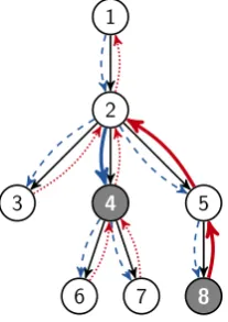
Therefore, our model performs the bottom-up pass first, and uses its output v↑ as the input for the top-down pass to obtain v↓. In this way, all tokens in the tree can be accessed by other tokens, since any two tokens have a common ancestor, and the information of one token can be first passed up to the common ancestor, then down to the other token. Figure 2 illustrates the information flow of our bidirectional model, where the red dotted arrows indicate the bottom-up pass, and the blue dashed arrows indicate the top-down pass. We highlight how node 8 influences node 4. Its rep-resentationv₈◦ is first propagated up to the lowest common ancestorv↑₂, then goes down tov↓₄.

1

2

3 4

6 7

5

8

Figure 2: An illustration of the information flow in the encoder, where the red dotted arrows represent the bottom-up pass and the blue dashed arrows represent the top-down pass. The solid arrows illustrate the in-formation flow from node 8 to node 4.

2.1.2 Head-First Decoder

We adopt the generaldivide-and-conquerstrategy as inBohnet et al.(2010), by first linearizing each subtree and then combining the ordered subtrees into a full sentence. Instead of generating the sequences from left to right as in Bohnet et al.

(2010), we generate the sequence from inside out, i.e., we initialize the sequence with the head, and expand outwards by appending the dependents to the left or the right end of the sequence.

This new generation order is motivated by the linguistic research on word order constraints, which largely focuses on the relative direction and distance of the dependent to the head (Gibson,

1998;Liu,2010;Gulordava,2018).

Following Bohnet et al. (2010), we use beam search to find the best sequence for each subtree incrementally, see the pseudocode in Algorithm1. We initialize the agenda with a sequence which contains only the head (line 3-4). A sequence is represented by two LSTMs, both initialized with the head representation, which corresponds to the left expansion and right expansion of the se-quence.

At each step, for each sequence in the agenda, we use a pointer network (Vinyals et al., 2015) to calculate the unnormalized attention score be-tween the left LSTM state and all the remaining tokens as the scores of attaching each token to the left (ATTENDl in line 101, wherevt is the vector representation of the token t), and we do the same for the right (line 14). We then create a new

se-1_{We actually calculate all attachment scores in one go, we}

quence for each possible attachment (line 9 and 13, where⊕denotes concatenation), and the score of each new sequence is incremented by the at-tachment score (line 10 and 14). We also update the corresponding LSTM state of that sequence by adding the representation of the attached depen-dent as input (line 11 and 15). The new sequences are then added into the agenda for the next step (line 12 and 16).

If the number of new sequences in the new agenda is larger than the beam size, we sort the sequences and keep only the highest scoring ones for further expansion (line 19-20), and we take the highest scoring full sequence as the linearization of the subtree (line 22). Finally, when each subtree is linearized, we combine them into a full sentence as the output (line 24).

Algorithm 1Head-first linearization 1: for allh∈T do

2: Th={h} ∪dependents(h) .subtree of headh

3: seq = [h] .initial sequence

4: agenda = [seq] .initial agenda

5: while|seq|<|Th|do

6: for allseq∈agendado

7: beam = []

8: for allt∈Th\seqdo .remaining tokens

9: seql= t⊕seq .attach left

10: seql.scorel+= ATTENDl(seq.statel,vt)

11: seql.statel= seq.statel.addInput(vt)

12: beam.append(seql)

13: seqr= seq⊕t .attach right

14: seqr.scorer+= ATTENDr(seq.stater,vt)

15: seqr.stater= seq.stater.addInput(vt)

16: beam.append(seqr)

17: end for 18: end for

19: SORTBYSCORE(beam)

20: agenda = N-BEST(beam, beam-size) 21: end while

22: Sh= N-BEST(agenda, 1) .best sequence for Th

23: end for

24: S = COMBINESUBTREES(S1, S2, ..., Sn)

25: returnS

We can easily modify the algorithm to left-to-right and left-to-right-to-left generation orders. Since the generation only goes in one direction, we only use one LSTM state to score the expansion, and the initial sequence is an empty sequence.

The three different decoders tend to make dif-ferent mistakes, since they have difdif-ferent starting points and could prune off the correct path in dif-ferent ways. Therefore it is beneficial to com-bine the three decoders to vote for the best se-quence. Concretely, we first shift the scores of the sequences in each beam so that the minimum score is 0 (implying that the absent sequences have

neg-ative scores), then combine the sequences from the three beams by summing up the scores for identi-cal sequences, and finally choose the highest scor-ing sequence in the combined beam as output.

2.1.3 Training with Beam Search

The head-first linearization introduces spurious ambiguity, since there may be two correct attach-ments (on the left or the right end of the sequence) at each step. Enforcing a canonical sequence of attachments would yield suboptimal performance. We view the order of attaching the dependents (i.e. whether to attach left or right dependent first) as latent variables, while the created sequence as the real target. We adopt the training method in

Bj¨orkelund and Kuhn(2014): at every step after pruning the beam, we check if there is still at least one gold partial sequence in the beam. If not, then we calculate the hinge loss between the highest scoring gold sequence andallincorrect sequences in the beam2.

We also follow the delayed LaSO strategy in

Bj¨orkelund and Kuhn (2014): after all gold par-tial sequences fall out of the beam and a loss is incurred, we continue training by putting the gold sequence back into the beam, until reaching the full sequence. This is shown to be more sample ef-ficient than the early-update strategy (Collins and Roark,2004), since it allows the model to train on the full sequence, even if the gold path falls out of the beam early.

The standard hinge loss updates the gold se-quence against the incorrect ones by enforcing a margin (typically 1), which punishes all incorrect sequences equally. However, not all incorrect se-quences are equally bad in terms of the BLEU score, therefore, maintaining a larger margin for worse sequences could improve the performance.

We cannot directly use BLEU score as the mar-gin, since it is calculated on the sentence level, while we are training on the subtree level, and the sequences in the training are often incomplete due to early-stop. Therefore, we use the inversion number as the surrogate loss for the BLEU score.

For a partial sequence, we first append the rest of the tokens to both ends of the sequence in the optimal way, then calculate the number of swaps in a bubble-sort to the gold sequence, and

2_{Perceptron-based training only updates against the}

take the squared root as the loss3. For exam-ple, if we have a predicted partial sequence of (1,2,4,6,7), and the remaining tokens are{3,5}, then we first obtain the best available full sequence (3,1,2,4,6,7,5), then calculate the number of swaps in a bubble-sort, which is 4, and the loss value is thus 2.

2.2 Inflection

We use a simple hybrid approach for the inflection task. We first extract all inflection patterns from the training data: given the combination of lemma, UPOS, and morphological features, if there is a word form appearing more than once and has over 99% certainty, then we keep it as a rule.

For the tokens not covered by the rules, we use a seq2seq model to predict the inflection similar toKann and Sch¨utze(2016), but with a major dif-ference. Instead of the inflected word, we predict the edit script that modifies the lemma to the word as the output sequence. The alphabet of the edit script includes all the characters in the treebank and three special symbols: 3 to copy one input character, 7 to delete one input character, and $ to finish generation. For example, to inflect the Portuguese verb “falar” to “falando”, the output sequence is “33337ndo$”. The advantage of predicting edit scripts instead of words is that the copy action avoids the mistake of generating in-correct but similar characters.

The edit script is in a way also similar toBohnet et al.(2010), but they predict the full edit scripts as one tag, which results in a very large tag set for many morphologically rich languages, and makes it difficult to learn and to generalize.

We use a bidirectional LSTM to encode the characters of the lemma and the morphological tags as a sequence. Each character embedding is concatenated with a binary feature that indicates whether the corresponding input character is cur-rently the target of the edit operation. Initially, the indicator for the first character is set to 1 and the rest are 0. A decoder LSTM with attention is then used to predict the edit operations. The input to the decoder LSTM state is the concatenation of the tree-structured token representation as in §2.1.1, the attended input vector, and the embedding of the last produced character4. If the predicted

ac-3

Since the complexity of bubble-sort isO(n2), we make it linear to avoid unstable loss values.

4_{In the case of copy, we use the embedding of the copied}

character instead of the copy symbol3.

tion is copy(3) or delete(7), the indicator on the input is then advanced by one step, and if the pre-diction is adding a character, the indicator does not move.

2.3 Detokenization

Since the surface realization shared task is eval-uated on the generated text instead of tokens, a detokenization step is needed to compare with other participant systems. We first contract the tokenized words into one token, for example in Portuguese, the preposition “de” and determiner “estes” are contracted into one token “destes” in the text.

We extract the contraction cases from the train-ing set, and construct an automaton to contract the tokens. Concretely, we read the tokens one by one, and when a token matches the initial state of the automaton, we store the token into a buffer and advance the automaton. If it reaches the end state, we replace the tokens in the buffer with the corre-sponding contracted token, otherwise we add the tokens in the buffer into the output sequence.

The final step is to remove the spaces surround-ing certain punctuation marks, e.g., the period at the end of the sentence. We use a rule-based off-the-shelf tool MosesDetokenizer5, which yields satisfactory results, compared to some other simi-lar alternatives.

3 Experiments

3.1 Data and Baselines

We conduct the experiments on the datasets from the previous Surface Realization Shared Task 2018 (SR18) (Belz et al., 2018), which includes 10 (mostly European) languages from the Univer-sal Dependencies (Nivre et al.,2016).

We compare our system with two state-of-the-art linearization systemsBohnet et al.(2010) and

Puduppully et al. (2016), referred to as B10 and P16. We run their linearization systemsas is, us-ing lemma, UPOS and dependency labels as fea-tures. We also use the same features in our system for comparison. To evaluate the linearization step alone, we calculate BLEU score based on lemma. We also compare to the best performing systems in the SR18, where the final BLEU score is re-ported on the detokenized text. We execute our

5_{https://pypi.org/project/}

full pipeline of linearization, inflection, and deto-kenization and evaluate with the official evalua-tion script. We also apply our inflecevalua-tion and deto-kenization steps on the predicted linearization of B10 and P16, so that they can also be compared to other systems.

3.2 Implementation Details

Our model is implemented with the DyNet Library (Neubig et al., 2017), and is available at the first author’s website6. We use the embedding sizes of 64, 32 and 32 for lemma, UPOS and depen-dency labels, respectively, and the dimension for the token representation is 128. The hidden states of both bottom-up and top-down encoder LSTMs, as well as the decoder LSTMs, have dimension of 128. The decoder beam size is 32. The linearizer is quite efficient among neural models, training a medium sized treebank takes about 2 hours on a single CPU core.

3.3 Linearization

We first compare each step in our pipeline to the available baselines. For linearization, we test our models with the same tree encoding and different decoding orders (left-to-right (L2R), right-to-left (R2L), head-first (H2LR), as well as voting among the three (Vote). The results are shown in Table1. Among the two baseline systems, B10 performs more than 4 BLEU points higher than P16, we believe the reason is that the subtree-level beam search in B10 allows it to explore almost all pos-sible permutations for most of the subtrees7, while P16 directly orders the full sentence, which can only explore a fraction of the full search space even with a very large beam size. Understandably, the P16 model is designed to linearize words with partial or even no syntactic information, there-fore the knowledge of subtrees cannot be assumed. However, in the scenario with full syntactic infor-mation available, B10 is clearly a better model.

We then compare our model to B10. The L2R linearizer generates the hypothesis in the same way as B10, and it uses a much smaller beam with the size of 32. It achieves 1 BLEU point higher than B10, which demonstrates the advantage of the more expressive tree-based representation.

6_{https://www.ims.uni-stuttgart.de/}

institut/mitarbeiter/xiangyu/

7_{They use beam size of 1000, which can cover all possible}

permutations of up to 6 tokens (6! = 720).

The H2LR order performs better than L2R and R2L, which could be explained in multiple as-pects. One explanation is our motivation that gen-erating from the head could better reflect word or-der constraints. The other explanation is that train-ing with latent generation order allows the model to make easier decision first, similar to the easy-first parser byGoldberg and Elhadad(2010).

Finally, when combining the three decoders to-gether by voting, it achieves 2 BLEU points higher than B10. There are two main reasons for this im-provement: (1) multitask-style training helps regu-larize the parameters, and (2) different generation directions tend to prune the correct sequences at different locations, and the mistake in one direc-tion might be saved by the other two.

B10 P16 L2R R2L H2LR Vote

ar 81.78 77.07 82.78 82.48 82.79 83.37 cs 74.74 70.93 73.52 71.89 74.16 75.17 en 82.83 78.80 84.92 83.95 84.01 85.48 es 81.84 74.33 82.82 82.53 82.99 83.69 fi 69.95 63.74 68.69 69.58 70.15 71.08 fr 84.38 81.74 85.04 85.24 85.45 85.66 it 82.60 77.41 83.03 83.28 82.66 84.51 nl 67.82 62.56 71.68 70.54 72.25 72.49 pt 80.46 76.52 81.48 81.13 82.10 81.80 ru 83.40 82.96 85.39 85.51 85.45 87.11

avg 78.98 74.61 79.94 79.61 80.20 81.04

Table 1: Linearization on the development set, where we compare different generation orders (L2R, R2L, H2LR and Voting) with Bohnet et al. (2010) and Puduppully et al.(2016).

3.4 Inflection

Table 2 shows the inflection performance with different models: the first model predicts edit script as a tag (EditTag); the second model pre-dicts the character sequence of the inflected word (CharSeq); the third model predicts the edit scripts as sequences of actions (EditSeq); and the last one uses the same model as the third, but first applies the extracted rules if available (+rule). The results are compared to the reported inflection accuracy inPuzikov and Gurevych (2018) (P18), which is adapted fromAharoni and Goldberg(2017).

P18 EditTag CharSeq EditSeq +rule

ar 93.07 88.02 95.57 95.33 95.01

cs 99.53 97.52 97.01 97.98 98.92

en 98.11 98.57 97.95 98.33 98.51

es 99.59 98.11 98.59 99.27 99.47

fi 95.46 82.54 92.16 93.13 95.06

fr 95.56 90.83 95.85 97.39 97.78

it 97.44 92.87 96.84 98.05 98.49

nl 95.68 93.38 94.53 94.57 95.36

pt 99.30 93.05 98.45 98.71 99.22

ru 98.22 94.58 95.86 96.42 97.47

avg 97.20 92.95 96.28 96.92 97.53

Table 2: Inflection on the development set, where we compare our different models with Puzikov and Gurevych(2018): tagging edit scripts (EditTag), gen-erating character sequences (CharSeq), gengen-erating edit script sequences (EditSeq), and apply the extracted rules (+rules).

better than the EditTag, especially on the lan-guages with very large edit scripts tag sets. The EditSeq model performs better than the character seq2seq model, mainly because the copy mecha-nism avoids many noisy generation errors. Some typical mistakes by CharSeq we find in English are “traveling”→“braveling” and “children”→ “thil-dren”, where some characters in the input lemma are confused with a similar one. Some typical mis-take by the EditSeq are “kidding”→“kiding” and “clashes”→“clashs”, where some necessary char-acters in the output are omitted.

Finally, the combination of the EditSeq model and extracted rules performs the best. On the de-velopment sets, the token coverage of the rules ranges from about 60% to 90% for different lan-guages, with over 99% accuracy, which means the majority of the inflection can be produced reliably and efficiently by simply looking up in a dictio-nary. The hybrid approach even outperforms the very strong baseline, although the seq2seq model alone is slightly weaker than the baseline, we be-lieve this simple trick could also benefit other in-flection models.

3.5 Detokenization

As the final step, we evaluate the performance of the detokenization, which includes contracting words and attaching punctuation. We use gold lin-earization and inflection as the input.

We separate the evaluation into two parts: for contraction, we evaluate the token-based BLEU score against the gold contraction on the UD de-velopment set; for the punctuation attachment, we

use the gold contracted word and evaluate with the official text-based BLEU score. We also evaluate the combined results where both contraction and detokenization are predicted.

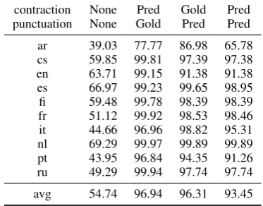
Table 3shows the results of these four scenar-ios. The first column contains the results of sim-ply separating all tokens with empty spaces. The BLEU score is around 55 even when the lineariza-tion and infleclineariza-tion are all correct, which shows the over-proportionally large impact of the deto-kenization in the shared task evaluation.

Our detokenizer works reasonably well for most of the languages, except for Arabic, where both contraction and detokenization results are rather poor. We will investigate this issue in the future work, it could potentially be addressed with a edit seq2seq model similar to the inflection task but on the sentence level.

contraction None Pred Gold Pred punctuation None Gold Pred Pred

ar 39.03 77.77 86.98 65.78 cs 59.85 99.81 97.39 97.38 en 63.71 99.15 91.38 91.38 es 66.97 99.23 99.65 98.95 fi 59.48 99.78 98.39 98.39 fr 51.12 99.92 98.53 98.46 it 44.66 96.96 98.82 95.31 nl 69.29 99.97 99.89 99.89 pt 43.95 96.84 94.35 91.26 ru 49.29 99.94 97.74 97.74

avg 54.74 96.94 96.31 93.45

Table 3: Detokenization on the development set, where the contraction and punctuation steps are gold, pre-dicted, or not used.

3.6 Final Results

We choose the best variant for each step in the pipeline for the full experiment, where we com-pare with the results from other participants in the shared task, as well as the linearizers of Bohnet et al. (2010) and Puduppully et al. (2016) com-bined with our inflection and detokenization mod-els as additional baselines for the shared task.

Table 4 shows the performance of the full pipeline on the test sets. B10 and P16 are the lin-earizers by Bohnet et al. (2010) and Puduppully et al. (2016) combined with our inflection and detokenization model, ST18 are the best results for each language in the shared task (King and White,

2018;Puzikov and Gurevych,2018;Ferreira et al.,

It is apparent that both B10 and P16 have higher performance than the other systems by a large margin. The advantage of our linearizer also car-ries over to the full pipeline, it scores 2 BLEU points higher than the best baseline.

B10 P16 ST18 Ours

ar 42.50 36.48 25.65 43.68 cs 64.75 58.87 25.05 65.42 en 70.75 65.86 69.14 72.67 es 74.75 56.50 65.31 77.77 fi 56.13 49.68 37.52 56.53 fr 66.62 52.12 52.03 68.75 it 69.09 47.14 44.46 71.98 nl 56.39 50.96 32.28 60.17 pt 66.13 49.34 30.82 66.16 ru 72.40 71.58 34.34 76.10

avg 63.95 53.85 41.66 65.92

Table 4: Final results on the test set, where we compare our model to two baselines (B10 and P16) and the best system in the shared task for each language (ST18).

4 Analysis

4.1 Relation Awareness

Our tree-based representation is theoretically able to propagate information from all other tokens in the tree. We now test whether it can really make use of such information.

We design a probing task to test whether the model can tell the relation between two tokens. Concretely, we pick two random tokens (t1,t2) in a tree, and their relation can be described as a tuple (d1, d2), which are the distances fromt1 andt2 to their common ancestor. For example in Figure2, the relation between token 4 and 8 is(1,2).

We build a simple MLP on the concatenation of the representations of both tokens to predict the relation as a classification task. To avoid data spar-sity, we only predictd1 andd2 up to 3, and all re-lations beyond this distance is classified class “too far”. There are in total4×4 = 16classes.

We test the token representations with and with-out tree encoding in two scenarios: (1) train all pa-rameters which tests whether the encoder architec-ture is able to learn the relations and (2) only train the MLP which tests whether the parametrized en-coder model actually captures such relation.

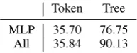
Table5shows the accuracy of the probing task. Clearly, the representation without tree encoding can not correctly classify the relation, its accuracy is higher than chance level because the lexical in-formation allows it to guess to some extent. The

Token Tree

MLP 35.70 76.75 All 35.84 90.13

Table 5: Relation classification accuracy of the en-coders with only token information (Token) vs. with tree information (Tree).

tree-structured encoder has much higher accuracy than the guessing baseline. Training on all param-eters achieves higher accuracy than only training on the MLP, which suggests that the encoder ar-chitecture is able to memorize the relation of many tokens, but the linearization task does not actually require that much information.

4.2 Synergy between Encoder and Decoder

Our model uses the bidirectional Tree-LSTM to pass information both bottom-up and top-down. However, it is not yet clear whether having both directions is necessary, and how much it would in-fluence the performance of different decoders.

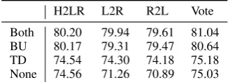
Table 6 shows the average performance of the four decoders (H2LR, L2R, R2L, and combining all) combined with four possible encoders: both directions (Both), only bottom-up (BU), only top-down (TD), and only token representation without tree information (None).

When no bottom-up pass is performed (TD and None), the performance drops by a large margin, which means that the information about the depen-dents is very crucial for linearization. In contrast, skipping the top-down pass has much smaller in-fluence on H2LR, while L2R and R2L also only have moderate performance drop.

Interestingly, the drop is much larger for L2R and R2L from only TD to None. The reason would be that L2R and R2L decoders treats each token equally and do not have any indication of the head if no structural information is used, while the H2LR decoder starts with the head and builds the sequence around it based on the head-oriented word order constraints. Therefore, even when there is no structural information, the prior in the H2LR decoder can still make better decisions. This also supports our intuition on the pivotal role of the head in the generation process.

H2LR L2R R2L Vote

Both 80.20 79.94 79.61 81.04 BU 80.17 79.31 79.47 80.64 TD 74.54 74.30 74.18 75.18 None 74.56 71.26 70.89 75.03

Table 6: Performance of combination of linearization orders and representations on the development set, av-eraged over 10 treebanks.

5 Conclusion

We present a dependency tree linearization model with tree-structured encoder and head-first de-coder, which outperforms the previous state-of-the-art linearizers. Combined with our morpho-logical inflection and detokenization model, it achieves the best performance on the Surface Re-alization Shared Task 2018 by a substantial mar-gin. We also show that the previous work by

Bohnet et al. (2010), which our decoding algo-rithm is based on, is still a very strong baseline.

As future work, we plan to extend the head-first linearization algorithm to (jointly) generate absent function words from the deep semantic represen-tation. It corresponds to the deep track of the sur-face realization shared tasks, which is also a more realistic setting for natural language generation.

Acknowledgements

This work was in part supported by funding from the Ministry of Science, Research and the Arts of the State of Baden-W¨urttemberg (MWK), within the CLARIN-D research project.

References

Roee Aharoni and Yoav Goldberg. 2017. Morpholog-ical Inflection Generation with Hard Monotonic At-tention. In Proceedings of the 55th Annual Meet-ing of the Association for Computational LMeet-inguistics (Volume 1: Long Papers), pages 2004–2015.

Srinivas Bangalore and Owen Rambow. 2000. Exploit-ing a Probabilistic Hierarchical Model for Genera-tion. InProceedings of the 18th conference on Com-putational linguistics-Volume 1, pages 42–48. Asso-ciation for Computational Linguistics.

Anja Belz, Michael White, Dominic Espinosa, Eric Kow, Deirdre Hogan, and Amanda Stent. 2011. The First Surface Realisation Shared Task: Overview and Evaluation Results. InProceedings of the 13th European workshop on natural language genera-tion, pages 217–226. Association for Computational Linguistics.

Anya Belz, Bernd Bohnet, Emily Pitler, Leo Wanner, and Simone Mille. 2018. The First Multilingual Surface Realisation Shared Task (SR’18): Overview and Evaluation Results.

Anders Bj¨orkelund and Jonas Kuhn. 2014. Learning Structured Perceptrons for Coreference Resolution with Latent Antecedents and Non-Local Features. In Proceedings of the 52nd Annual Meeting of the Association for Computational Linguistics (Volume 1: Long Papers), volume 1, pages 47–57.

Bernd Bohnet, Simon Mille, Benoˆıt Favre, and Leo Wanner. 2011. StuMaBa: From deep representa-tion to surface. In Proceedings of the 13th Eu-ropean workshop on natural language generation, pages 232–235.

Bernd Bohnet, Leo Wanner, Simon Mille, and Ali-cia Burga. 2010. Broad Coverage Multilingual Deep Sentence Generation with a Stochastic Multi-Level Realizer. In Proceedings of the 23rd Inter-national Conference on Computational Linguistics, pages 98–106. Association for Computational Lin-guistics.

John Carroll, Ann Copestake, Dan Flickinger, and Vic-tor Poznanski. 1999. An Efficient Chart Generator for (Semi-) Lexicalist Grammars. In Proceedings of the 7th European workshop on natural language generation (EWNLG99), pages 86–95.

Danqi Chen and Christopher Manning. 2014. A Fast and Accurate Dependency Parser Using Neural Net-works. In Proceedings of the 2014 conference on empirical methods in natural language processing (EMNLP), pages 740–750.

Michael Collins and Brian Roark. 2004. Incremental Parsing with the Perceptron Algorithm. In Proceed-ings of the 42nd Annual Meeting on Association for Computational Linguistics, page 111. Association for Computational Linguistics.

Ryan Cotterell, Christo Kirov, John Sylak-Glassman, David Yarowsky, Jason Eisner, and Mans Hulden. 2016. The SIGMORPHON 2016 Shared TaskMor-phological Reinflection. InProceedings of the 14th SIGMORPHON Workshop on Computational Re-search in Phonetics, Phonology, and Morphology, pages 10–22.

Henry Elder and Chris Hokamp. 2018. Generating High-Quality Surface Realizations Using Data Aug-mentation and Factored Sequence Models. In Pro-ceedings of the First Workshop on Multilingual Sur-face Realisation, pages 49–53.

Michael Elhadad and Jacques Robin. 1992. Control-ling Content Realization with Functional Unification Grammars. In International Workshop on Natural Language Generation, pages 89–104. Springer.

Proceedings of the First Workshop on Multilingual Surface Realisation, pages 35–38.

Katja Filippova and Michael Strube. 2009. Tree Lin-earization in English: Improving Language Model Based Approaches. InProceedings of Human Lan-guage Technologies: The 2009 Annual Conference of the North American Chapter of the Association for Computational Linguistics, Companion Volume: Short Papers, pages 225–228. Association for Com-putational Linguistics.

Richard Futrell, Kyle Mahowald, and Edward Gib-son. 2015. Quantifying Word Order Freedom in Dependency Corpora. In Proceedings of the third international conference on dependency linguistics (Depling 2015), pages 91–100.

Edward Gibson. 1998. Linguistic Complexity: Local-ity of Syntactic Dependencies. Cognition, 68(1):1– 76.

Yoav Goldberg and Michael Elhadad. 2010. An Effi-cient Algorithm for Easy-First Non-Directional De-pendency Parsing. In Human Language Technolo-gies: The 2010 Annual Conference of the North American Chapter of the Association for Computa-tional Linguistics, pages 742–750. Association for Computational Linguistics.

Alex Graves and J¨urgen Schmidhuber. 2005. Frame-wise Phoneme Classification with Bidirectional LSTM and other Neural Network Architectures. Neural networks, 18(5-6):602–610.

Kristina Gulordava. 2018. Word Order Variation and Dependency Length Minimisation: A Cross-Linguistic Computational Approach. Ph.D. thesis, University of Geneva.

Wei He, Haifeng Wang, Yuqing Guo, and Ting Liu. 2009. Dependency Based Chinese Sentence Re-alization. In Proceedings of the Joint Conference of the 47th Annual Meeting of the ACL and the 4th International Joint Conference on Natural Lan-guage Processing of the AFNLP: Volume 2-Volume 2, pages 809–816. Association for Computational Linguistics.

Sepp Hochreiter and J¨urgen Schmidhuber. 1997. Long Short-Term Memory. Neural Comput., 9(8):1735– 1780.

Katharina Kann and Hinrich Sch¨utze. 2016. MED: The LMU system for the SIGMORPHON 2016 shared task on morphological reinflection. InProceedings of the 14th SIGMORPHON Workshop on Computa-tional Research in Phonetics, Phonology, and Mor-phology, pages 62–70.

David King and Michael White. 2018. The OSU Re-alizer for SRST ’18: Neural Sequence-to-Sequence Inflection and Incremental Locality-Based Lin-earization. InProceedings of the First Workshop on Multilingual Surface Realisation, pages 39–48.

Irene Langkilde and Kevin Knight. 1998. Genera-tion that Exploits Corpus-based Statistical Knowl-edge. In Proceedings of the 36th Annual Meet-ing of the Association for Computational LMeet-inguis- Linguis-tics and 17th International Conference on Compu-tational Linguistics-Volume 1, pages 704–710. As-sociation for Computational Linguistics.

Benoit Lavoie and Owen Rainbow. 1997. A Fast and Portable Realizer for Text Generation Systems. In Fifth Conference on Applied Natural Language Pro-cessing.

Haitao Liu. 2010. Dependency Direction as a Means of Word-Order Typology: A Method Based on De-pendency Treebanks.Lingua, 120(6):1567–1578.

Yijia Liu, Yue Zhang, Wanxiang Che, and Bing Qin. 2015. Transition-Based Syntactic Linearization. In Proceedings of the 2015 Conference of the North American Chapter of the Association for Computa-tional Linguistics: Human Language Technologies, pages 113–122.

Makoto Miwa and Mohit Bansal. 2016. End-to-End Relation Extraction using LSTMs on Sequences and Tree Structures. In Proceedings of the 54th An-nual Meeting of the Association for Computational Linguistics (Volume 1: Long Papers), pages 1105– 1116.

Graham Neubig, Chris Dyer, Yoav Goldberg, Austin Matthews, Waleed Ammar, Antonios Anastasopou-los, Miguel Ballesteros, David Chiang, Daniel Clothiaux, Trevor Cohn, et al. 2017. Dynet: The Dynamic Neural Network Toolkit. arXiv preprint arXiv:1701.03980.

Joakim Nivre, Marie-Catherine De Marneffe, Filip Ginter, Yoav Goldberg, Jan Hajic, Christopher D Manning, Ryan McDonald, Slav Petrov, Sampo Pyysalo, Natalia Silveira, et al. 2016. Universal De-pendencies v1: A Multilingual Treebank Collection. In Proceedings of the Tenth International Confer-ence on Language Resources and Evaluation (LREC 2016), pages 1659–1666.

Ratish Puduppully, Yue Zhang, and Manish Shrivas-tava. 2016. Transition-based Syntactic Lineariza-tion with Lookahead Features. InProceedings of the 2016 Conference of the North American Chapter of the Association for Computational Linguistics: Hu-man Language Technologies, pages 488–493.

Ratish Puduppully, Yue Zhang, and Manish Shrivas-tava. 2017. Transition-Based Deep Input Lineariza-tion. InProceedings of the 15th Conference of the European Chapter of the Association for Compu-tational Linguistics: Volume 1, Long Papers, vol-ume 1, pages 643–654.

Linfeng Song, Yue Zhang, and Daniel Gildea. 2018. Neural Transition-based Syntactic Linearization. In Proceedings of the 11th International Conference on Natural Language Generation, pages 431–440, Tilburg University, The Netherlands. Association for Computational Linguistics.

Kai Sheng Tai, Richard Socher, and Christopher D Manning. 2015. Improved Semantic Representa-tions From Tree-Structured Long Short-Term Mem-ory Networks. InProceedings of the 53rd Annual Meeting of the Association for Computational Lin-guistics and the 7th International Joint Conference on Natural Language Processing (Volume 1: Long Papers), volume 1, pages 1556–1566.

Oriol Vinyals, Meire Fortunato, and Navdeep Jaitly. 2015. Pointer Networks. InAdvances in Neural In-formation Processing Systems, pages 2692–2700.

Jie Zhou, Ganqu Cui, Zhengyan Zhang, Cheng Yang, Zhiyuan Liu, and Maosong Sun. 2018. Graph Neu-ral Networks: A Review of Methods and Applica-tions. arXiv preprint arXiv:1812.08434.