An Approach to Quantify the Loss Reduction due to
Distributed Generation
S B Karajgi
Department of Electrical Engineering S.D.M. College of Engineering and Technology,
Dharwad,India
Udaykumar R.Y
Department of Electrical Engineering National Institute of Technology Karnataka,
Surathkal,India
ABSTRACT
Line Loss Reduction is one of the major benefits of Distributed Generation, amongst many others, when incorporated in the Power Distribution System. The quantum of the line loss reduction should be exactly known to assess the effectiveness of the distributed generation. In this paper, the total loss of a practical distribution system is calculated with and without distributed generation and an index, quantifying the total line loss reduction is proposed. Simulation tests have been carried out on a practical distribution system and the proposed index is evaluated for various ratings, locations of distributed generation.
Keywords
Distributed Generation, System Loss Reduction Index.
1.
INTRODUCTION
The presence of Distributed Generation (DG) has been shown to be beneficial in many respects like voltage profile improvement, line loss reduction, improvement in reliability etc. [1]-[5]. The evaluation of these benefits is very critical in assessing the merit of DG. The quantification of the benefit of line loss reduction was proposed in [6], which evaluated the line losses both with and without DG and the benefit index was defined as the ratio of line loss with DG and that without DG. The subsequent researches [7]-[10], also defined the quantification in a similar way and the benefits of DG were defined. These works, however, considered only the losses in the lines and the quantification was defined for the line losses only. These indices, therefore, do not indicate the loss reduction of the system itself. A practical distribution system consists of several distribution transformers, supplying consumers at low voltage on the secondary side. The losses occurring in these transformers and the line losses of the secondary low voltage distribution system should also be considered to arrive at the overall loss reduction of the system. In this paper, a practical distribution system, supplying a number of consumers at low voltage, is considered. The losses occurring in the transformers and the low voltage distribution lines have been considered and the benefit of DG in respect of total loss is evaluated.
2.
DESCRIPTION OF THE SYSTEM
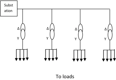
A simple distribution system shown in fig 1, is considered for analysis. The system consists a number of identical
distribution transformers, the secondary of which supply power to the consumers at low voltage. The core loss 0f each transformer is represented by Pc.
Fig 1: The single line diagram of a standard distribution
system.
For simplicity, the following assumptions are made.
All loads are modeled as constant current loads, drawing the same current irrespective of the
respective voltages.
The core losses of the transformers remain constant at a value depending on the rating.
All loads draw the power at a power factor of 0.8 lagging.
DG unit is capable of supplying power at both leading and lagging power factors.
The copper losses of the distribution transformer are of small value and are neglected
3.
LOSS REDUCTION ANALYSIS
The total loss of the distribution system without DG is
given by Subst ation
∆
Y
To loads
∆Y
∆
Y
∆
[image:1.595.315.550.287.449.2]Loss Syst w/o DG =
1 1 1 1 2 N i LV C N i ii
rl
P
iP
iI
(1)Where I is the current flowing through ith segment ,L i is
the length of ith segment, r is the resistance of line in ohms per unit length., is the core loss of ith transformer, is the Losses on the low voltage side of
the ith transformer and N is the number of busses in the system.
In order to determine the losses of the system, the core
loss of each transformer and the LV side losses on each
transformer must be known. It is evident from the above
equation that the total losses can be reduced only by
reducing the first term of equation (4.1) which represents
the feeder line losses, since the other term representing
the core loss and the LV side loss of each transformer
remain same independent of the presence of DG.
With the inclusion of DG, the currents in the feeder
segments will be redistributed. If a DG unit is inserted at
Kth bus, the feeder segments up to bus K will carry the difference of the initial current and the injected current
by the DG unit. The segments beyond K will continue to
carry the same currents. The total loss of the feeder with
DG is the given by
Loss Feed w DG = i
N K i i K i i G
i
I
rl
I
rl
I
1 21
1
2
)
(
(2)Where is the current injected by the DG unit and
remains the same at earlier value.
The total loss of the distribution system with DG is
now
LossSystwDG=
1 1 1 2 1 1 2)
(
N i LV C i N K i i K i i Gi
I
rl
I
rl
P
iP
iI
(3)A factor, System Loss Reduction Index (SLRI), which
quantifies the loss reduction with the insertion of DG is
defined as
SLRI = Loss in the system with DG
Loss in the system without DG
=
1 1 1 2 1 1 2)
(
N i LV C i N K i i K i i Gi
I
rl
I
rl
P
iP
iI
i N K i i K i i Gi
I
rl
I
rl
I
1 21
1
2
)
(
(4)The distribution system loss can be rewritten as
LossSyswDG=
1 11 2 2 1 1 2
2
N K i N i LV C i i i K i G G ii
I
I
I
rl
I
rl
P
iP
iI
=
1 1 1 1 2 1 1 2)
2
(
N i N i LV C i i i K i G iG
I
I
rl
I
rl
P
iP
iI
(5)
Substituting equation (2) in equation (5) we get
LossSystwDG = LossSystw/o DG + ∑ ( ) (6)
On simplification, following equation is obtained
Loss Syst w DG = Loss Syst w/o DG +
iK
i
i G
G
I
I
rl
I
1 12
= Loss Syst w/o DG + Kloss IG (7)
Where Kloss is the loss factor given by
Kloss =
iK
i
i
G
I
rl
I
1 12
(8)The SLRI is now obtained as
SLRI = = Loss Syst w/o DG + Kloss IG (9)
Loss Syst w/o DG
If SLRI < 1 , the DG has reduced the losses and is beneficial
= 1the DG has not made any changes in the system.
1, the DG has introduced more losses in the system.
It is clear from equation (9) that the loss factor Kloss
must be negative if DG is expected to reduce the losses in the
system. Since the loss factor depends on the summation of
the difference between the injected DG current and twice the
feeder segment current, it attains maximum negative value
The Loss factor and thus the SLRI are greatly influenced by the power factors of the DG unit. In case the unit is operating at unity power factor, all the reactive power required by the load is supplied by the source and hence the there may not be any appreciable decrease of line current supplied by the source leading to higher losses and thus low SLRI.
4.
SIMULATION TESTS
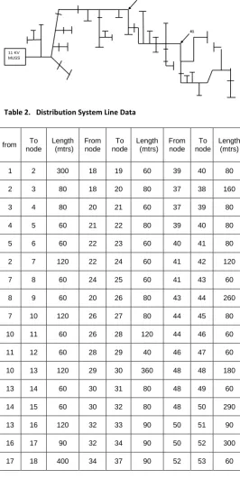
A practical 36 bus, 11 KV distribution feeder shown in fig 2,
is considered. The system consists of 35 distribution
transformers with various ratings. The details of the
distribution transformers are given in table 1. The base MVA
used in the study is 5 MVA. The conductor used is Rabbit
with resistance of 0.0030173 pu/km and reactance of 0.
0020143 pu/km. The lengths of the feeder segments are given
in table 2. The total connected load on the system is 2300
KVA and the peak demand for the year is 2000 KVA at a pf
of 0.8 lag. The connected loads on the transformers are listed
in table 3.
The system consists of two DG units described below.
1. DG1, of rating 270 KW, connected at node No 26,
shown with arrow mark in the fig.2.
2. DG2, of rating 800 KW connected at node No 41,
shown with arrow mark in fig 2.
Table 1. Details of transformers in the system
Fig 2: Single line Diagram of the distribution system
[image:3.595.311.578.238.770.2]
Table 2. Distribution System Line Data
from To node
Length (mtrs)
From node
To node
Length (mtrs)
From node
To node
Length (mtrs)
1 2 300 18 19 60 39 40 80
2 3 80 18 20 80 37 38 160
3 4 80 20 21 60 37 39 80
4 5 60 21 22 80 39 40 80
5 6 60 22 23 60 40 41 80
2 7 120 22 24 60 41 42 120
7 8 60 24 25 60 41 43 60
8 9 60 20 26 80 43 44 260
7 10 120 26 27 80 44 45 80
10 11 60 26 28 120 44 46 60
11 12 60 28 29 40 46 47 60
10 13 120 29 30 360 48 48 180
13 14 60 30 31 80 48 49 60
14 15 60 30 32 80 48 50 290
13 16 120 32 33 90 50 51 90
16 17 90 32 34 90 50 52 300
17 18 400 34 37 90 52 53 60
41 26
11 KV MUSS
Rating (KVA) 63 100 250
Number 16 18 1
No Load Losses (Watts) 180 260 470
Table 3. Details of the connected loads.
Transformer
No
Load in
KVA
Transformer
No
Load in
KVA
1 61 19 61
2 61 20 61
3 38 21 61
4 38 22 38
5 38 23 38
6 38 24 61
7 38 25 61
8 38 26 38
9 38 27 38
10 61 28 61
11 38 29 61
12 61 30 61
13 61 31 61
14 38 32 38
15 61 33 38
16 38 34 61
17 61 35 153
18 61
5.
METHOD OF STUDY
Following steps are followed to evaluate the impacts of DG
on the system loss reduction and also to quantify the proposed
index.
The power outputs of both DG1 and DG2 are fixed. The details of the distribution system are collected
and the system is simulated using CYMEDIST
computer simulation program and the DG units are
incorporated in the simulated system.
Load flow studies are conducted for all the specified cases and the results are obtained.
The results are analyzed and the impacts of DG on the loss reduction are evaluated.
Specific cases considered for study:
The impact of DG in respect of Line Loss
Improvement is studied with and without DG in the system.
The operating power factor of DG1 is kept constant at unity
and that of DG2 is varied from 0.8 lag, 0.9 lag, unity, 0.9 lead
and 0.8 lead. While carrying out the tests, the following
assumptions are made.
All the loads draw power at 0.8 lagging.
The loads on the low voltage side are distributed over line of length 300 mtrs.
The core losses of the transformers remain constant at their rated value.
6.
RESULTS
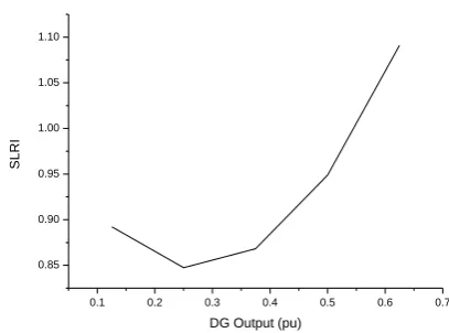
The simulation results are given in figure 3. These results
reveal that the inclusion of DG reduce the line losses as
expected. It can be shown from the graphs that, SLRI
decreases marginally, since the core losses of the transformers
and the LV side losses remain constant being independent of
the presence of DG. This is an improvement over the index
derived in [6], which considered only the feeder line losses. It
can also be seen that with the increase in the DG output,
SLRI, decrease but again show an increasing trend after a
threshold value e.g. as the power output is increased the SLRI
starts increasing as shown in fig.4. This is because the system
receives more power from DG than required and hence the
line loss increase appreciably. This should be considered
before fixing up the value of DG output. Under such a case,
one DG unit can be switched off so that the advantage of
lower SLRI can be enjoyed.
The operating power factor of DG also influences the SLRI.
It is very clear from the fig 5 that SLRI has lower values with
DG operating at lagging power factor and increase under
leading power factor. This is because the DG unit absorbs
reactive power from the lines under leading power factor.
Further, it can be seen that the index may exceed unity,
indicating that the presence of DG has increased the line
losses than decreasing it. This factor should be considered
while fixing the operating power factor of DG.
The variation of loss factor is shown in fig. 6. It is clear from
the loss reduction depends mainly on the current injected by
the DG unit. When IG is more than IL, loss factor becomes
positive and the total losses in the system increase, leading
SLRI to acquire a value greater than one.
The location of DG is also very critical in deciding the loss
reduction. It is evident from figure 7, that SLRI show a
decreasing trend when DG is located away from the
substation. This issue should be considered before installing
DG in the system.
0.1 0.2 0.3 0.4 0.5 0.6 0.7
0.70 0.75 0.80 0.85 0.90 0.95
SLR
I
DG Output (pu)
Fig 3: Variation of SLRI with DG Output
0.8 Lag 0.9 Lag UPF 0.9 Lead 0.8 Lead
0.70 0.75 0.80 0.85 0.90 0.95 1.00 1.05
SLR
I
[image:5.595.325.529.78.229.2]Operating power factor of DG2
Fig 4: Variation of SLRI with operating power factor of DG
0.1 0.2 0.3 0.4 0.5 0.6 0.7
0.85 0.90 0.95 1.00 1.05 1.10
SLR
I
DG Output (pu)
Fig 5: Variation of SLRI with high penetration of DG
0.00 0.02 0.04 0.06 0.08 0.10 0.12 0.14 0.16 0.18 0.20
0.0 -0.2 -0.4 -0.6 -0.8 -1.0
L
o
ss
fa
ct
o
r
DG Output (pu)
Fig 6: Variation of Loss Factor with DG output.
0.02 0.04 0.06 0.08 0.10 0.12 0.14 0.16 0.18
0.86 0.88 0.90 0.92 0.94 0.96 0.98
SLR
I
DG Out put (pu)
DG connected at node 26 DG connected at node 41
Fig 7: Variation of SLRI with the same DG connected at
7.
CONCLUSION
The simulation results show that the inclusion of DG,
marginally reduce the losses in a distribution system. This is
because; the line losses form only a minor part of the
distribution system losses and the DG can reduce only the line
losses. The other losses viz. the transformer losses and the LV
side distribution losses remain unaltered. Hence this fact
should be considered before installing a DG into a system.
8.
REFERENCES
[1] T. Ackermann, G. Andersson, and L. Soder, “Distributed generation: A definition,” Elect. Power Syst. Res., vol. 57, pp. 195–204, 2001.
[2] N. Hadjsaid, J. Canard, and F. Dumas, “Dispersed generation impact on distribution networks,” IEEE Comput. Appl. Power, vol. 12, no. 2, pp. 22–28, Apr. 1999.
[3] Peter. Daly, “ Understanding the potential Benefits of DG on Power Delivery System”, a paper presented at Rural Electric Power conference 2001, Little Rock, Arkansas, 2001.
[4] Ahmed Azmy, “ Impact of DG on the Stability of Electrical Power Systems”, ”, IEEE Trans. On Power Delivery, 2005, pp 1 – 8
[5] E. Vidyasagar, P.V.N.Prasad, “Impact of DG on Radial Distribution System Reliability”, in 15th National Power System Conference Conference (NPSC), IIT Bombay 2008, pp 467-472
[6] P. Chiradeja, “Benefit of distributed generation: A line loss reduction analysis,” in Proc. IEEE-Power Eng. Soc. Transmission and Distribution Conf. Exhib.: Asia and Pacific, Dalian, China, Aug. 15–17, 2005.
[7] Chiradeja, Ramkumar , “ An Approach to quantify the Benefits of Distrributed Generation Systems”, IEEE trans. On Energy Conversion, Vol. 19, Dec 2004, pp 764 – 773.
[8] M.A.Kashem , M.Negnevitsky , G.Ledwich , "
Distributed Generation for minimization of power losses in distribution systems " , IEEE conference 2006 [9] Hugo A. Gil, Geza Joos,” Models for Quantifying the
Economic Benefits of Distributed Generation”, IEEE TRANSACTIONS ON POWER SYSTEMS, VOL. 23, NO. 2, MAY 2008,pp327-335