Linear Dimension Reduction for Multiple Heteroscedastic Multivariate Normal Populations

(1)

http://dx.doi.org/10.4236/ojs.2015.54033

Linear Dimension Reduction for

Multiple Heteroscedastic Multivariate

Normal Populations

Songthip T. Ounpraseuth

1

, Phil D. Young

2

, Johanna S. van Zyl

2

,

Tyler W. Nelson

2

_{, Dean M. Young}

2

1_{Department of Biostatistics, University of Arkansas for Medical Sciences, Little Rock, AK, USA} 2_{Department of Statistical Science, Baylor University, Waco, TX, USA}

Email: [email protected], [email protected], [email protected],

[email protected], [email protected]

Received 16 April 2015; accepted 19 June 2015; published 24 June 2015

This work is licensed under the Creative Commons Attribution International License (CC BY).

http://creativecommons.org/licenses/by/4.0/

Abstract

For the case where all multivariate normal parameters are known, we derive a new linear dimen-sion reduction (LDR) method to determine a low-dimendimen-sional subspace that preserves or nearly preserves the original feature-space separation of the individual populations and the Bayes pro- bability of misclassification. We also give necessary and sufficient conditions which provide the smallest reduced dimension that essentially retains the Bayes probability of misclassification from the original full-dimensional space in the reduced space. Moreover, our new LDR procedure requires no computationally expensive optimization procedure. Finally, for the case where para-meters are unknown, we devise a LDR method based on our new theorem and compare our LDR method with three competing LDR methods using Monte Carlo simulations and a parametric boot-strap based on real data.

Keywords

Linear Transformation, Bayes Classification, Feature Extraction, Probability of Misclassification

1. Introduction

(2)

large relative to the training-sample sizes, the performance or efficacy of a sample discriminant rule may be considerably degraded. This phenomenon gives rise to a paradoxical behavior that [1] has called the curse of dimensionality.

An exact relationship between the expected probability of misclassification (EPMC), training-sample sizes, feature-space dimension, and actual parameters of the class-conditional densities is challenging to obtain. In general, as the classifier becomes more complex, the ratio of sample size to dimensionality must increase at an exponential rate to avoid the curse of dimensionality. The authors [2] have suggested a ratio of at least ten times as many training samples per class as the feature dimension increases. Hence, as the number of feature variables

p becomes large relative to the training-sample sizes n_i, i=1,,m, where m is the number of classes, one might wish to use a smaller number of the feature variables to improve the classifier performance or computa-tional efficiency. This approach is called feature subset selection.

Another effective approach to obtain a reduced dimension to avoid the curse of dimensionality is linear di-mension reduction (LDR). Perhaps the most well-known LDR procedure for the m-class problem is linear dis-criminant analysis (LDA) from [3], which is a generalization of the linear discriminant function (LDF) derived in [4] for the case m=2. The LDA LDR method determines a vector

a

that maximizes the ratio of between- class scatter to average within-class scatter in the lower-dimensional space. The sample within-class scatter matrix is

1 ,

m

W i i

i α

=

≡

∑

S S (1)

where S_i is the estimated sample covariance matrix for the ith class, and the sample between-class scatter ma-trix is

(

)(

)

1

,

m

B i i i

i α

=

′

≡

∑

− −

S x x x x (2)

where x_i is the sample mean vector for class Π_i, α_i is its a priori probability of class membership,

1 m

i i i=α

=

∑

x x is the estimated overall mean, and i=1,,m. For m=2 with α₁=α₂, [4] determined the vector

a

that maximizes the criterion function

( ) (

B

)

,

F

W ′ =

′

a S a

J a

a S a

which is achieved by an eigenvalue decomposition of 1

W B

−

S S . An attractive feature of LDA as a LDR method is that it is computationally appealing; however, it attempts to maximally separate class means and does not in-corporate the discriminatory information contained in the differences of the class covariance matrices. Many al-ternative approaches to the LDA LDR method have been proposed. For example, canonical variables can be viewed as an extension to the LDF when m>2 and q>1 (see [5]). Other straightforward extensions of the

LDF include those in [6] [7].

Extensions of LDA that incorporate information on the differences in covariance matrices are known as hete-roscedastic linear dimension reduction (HLDR) methods. The authors [8] have proposed an eigenvalue-based

HLDR approach for m>2, utilizing the so-called Chernoff criterion, and have extended the well-known LDA

method using directed distance matrices that can be considered a generalization of (2). Additional HLDR me-thods have been proposed by authors such as [9]-[10].

Using results by [13] that characterize linear sufficient statistics for multivariate normal distributions, we develop an explicit LDR matrix B∈_{q p}_× such that

,

→ =

x y Bx

where x∈_p_×₁, y∈_q_×₁, and _{m n}_× denotes the space of all

m n

×

real matrices. Using the Bayes classifi-cation procedure in which we assume equal costs of misclassificlassifi-cation and that all class parameters are known, we determine the reduced dimension q< p that is the smallest reduced dimension for which there exists a

(3)

corres-ponding Bayes classification rule assigns Bx to Π_k, where k∈

{

1,,m

}

. We refer to this method as the SY LDR procedure.

Moreover, we use Monte Carlo simulations to compare the classification efficacy of the BE method, sliced inverse regression (SIR), and sliced average variance estimation (SAVE) found in [14]-[16], respectively, with the SY method.

The remainder of this paper is organized as follows. We begin with a brief introduction to the Bayes quadratic classifier in Section 2 and introduce some preliminary results that we use to prove our new LDR method in Sec-tion 3. In SecSec-tion 4, we provide condiSec-tions under which the Bayes quadratic classificaSec-tion rule is preserved in the low-dimensional space and derive a new LDR matrix. We establish a SVD-based approximation to our LDR

procedure along with an example of low-dimensional graphical representations in Section 5. We describe the four LDR methods that we compare using Monte Carlo simulations in Section 6. We present five Monte Carlo simulations in which we compare the competing LDR procedures for various population parameter configura-tions in Section 7. In Section 8, we compare the four methods using bootstrap simulaconfigura-tions for a real data exam-ple, and, finally, we offer a few concluding remarks in Section 9.

2. The Bayes Quadratic Classifier

The Bayesian statistical classifier discriminates based on the probability density functions p

(

Π_i x

)

, i=1,,m, of each class. The Bayes classifier is optimal in the sense that it maximizes the class a posteriori probability provided all class distributions and corresponding parameters are known. That is, suppose we have m classes,

1, , m

Π _ Π , with assumed known a priori probabilities α₁,,αm, respectively. Also, let p

(

⋅ Πi

)

denote the

p-dimensional multivariate normal density corresponding to population Π_i, i=1,,m. The goal of statistical decision theory is to obtain a decision rule that assigns an unlabeled observation x to Π_k if p

(

Π_k x

)

is the maximum overall a posteriori p

(

Π_i x

)

, i=1,,m. Then,

(

)

0,

, 1,

i j

i j i j λ _{Π Π = } =

≠ 

the Bayes classifier assigns

x

to class Π_k if

(

k

)

(

j

)

, 1, , ; .

p Π x > p Π x j=  m j≠k

This decision rule partitions the measurement or feature space into m disjoint regions i

RΠ , where i=1,,m,

such that

x

is assigned to class Π_k if k RΠ

∈

x . Using Bayes’ rule, the a posteriori probabilities of class membership p

(

Π_k x

)

can be defined as

(

_k

)

kp

(

_{( )}

k

)

.

p

α Π

Π x = x

x

One can re-express the Bayes classification as the following: Assign

x

to Π_k if

(

)

(

)

, 1, , ; . kp k jp j j m j k

α xΠ >α xΠ =  ≠ (3)

This decision rule is known as the Bayes’ classification rule. Let Π_i be modeled as a p-dimensional multi-variate normal distribution, and let

( )

( ) (

)

1

(

)

ln 2 ln , 1, , .

i i i i i i

d x ≡ Σ − _

α

_+ x−

µ

′Σ− x−

µ

i=  m (4) The Bayes decision rule (4) is to classify the unlabeled observation

x

into the class Π_k such that

( )

min

{

( )

; 1, ,

}

k i

d x = d x i=  m . The classification rule defined by (4) is known as the quadratic discriminant function (QDF), or the quadratic classifier.

3. Preliminary Results

The following notation will be used throughout the remainder of the paper. We let p

>

(4)

positive definite matrices and S_{p p}_× denote the set of p×p symmetric matrices. Also, we let A+∈_{m n}_×

represent the Moore-Penrose pseudo-inverse of A∈_{n m}_× .

The proof of the main result for the derivation of our new LDR method requires the following notation and lemmas. Let M∈_p_{× −}₍_m₁₎₍_p₊₁₎ be

[

2 1| | m 1| 2 1| | m 1

]

,

≡ − _ − − _ −

T d d d d E E E E (5)

where d_i∈_p_×₁, Ei∈Sp p× such that rank

( )

Ei = p, and d1≠dk and E1≠Ek for at least one value of k, where 2≤ ≤k m and i=1,,m. Also, let rank

( )

T = ≤ <1 q p, and let F∈_{p q}_× and G∈_q_{× −}₍_m₁₎₍_p₊₁₎ be matrix components of a full-rank decomposition of T so that T =FG with rank

( )

F =rank

( )

G =q. Then, the Moore-Penrose pseudoinverse of T is T+ =G F+ +, and, also, TT+ =FF+ and TT T+ =FF T+ =T. This result implies that for i=1,,m,

(i)

(

I−FF+

)

(

d_i−d₁

)

=0 and (ii)

(

I−FF+

)

(

E_i−E₁

)

=0.

We now state and prove three lemmas that we use in the proof of our main result.

Lemma 1 For T =FG in (5), where E_i∈S_{p p}_× , d_i∈_p_×₁, F∈_{p q}_× , and G∈_q_{× −}₍_m ₁₎₍_p₊₁₎ such that

( )

rank F =rank G =q, and i=1,,m, we have that

(a) FF+

(

E_i−E₁

) (

= E_i−E FF₁

)

+, (b) FF E+ _i =E FF_i +, and

(c)

(

I−FF+

)

E_i =E I₁

(

−FF+

)

.

Proof. Part (a) follows from the fact that E_i =E_i′, i=1,,m, and from (ii) above. Parts (b) and (c) follow directly from (a).

Lemma 2 For T =FG in (5), where E_i∈S_{p p}_× , d_i∈_p_×₁, F∈_{p q}_× , and G∈_q_{× −}₍_m ₁₎₍_p₊₁₎ such that

( )

rank F =rank G =q, and i=1,,m, we have that

1

i i

−

+ + −

 ′ ₌ _′

F E F  F E F .

Proof. Because F E F+ _i +′ ∈_{q q}_× and rank

(

F E F+ _i +′ =

)

q, the result follows because

(

)

(

1

)

1 1 _.

i i i i i i q

+ +′ _′ − ₌ + _ +_ − ₌ + + − ₌

 

F E F F E F F E FF E F F FF E E F I

Lemma 3 Let T =FG in (5), where Ei∈Sp p× , di∈p×1, F∈p q× and G∈q× −(m 1)(p+1) such that

( )

rank F =rank G =q, and i=1,,m. Also, let C=R I_ −FF+_∈₍_{p q}_{− ×}₎ _p, where R∈₍_{p q}_{− ×}₎ _p such that rank

( )

C = −p q. Then,

(a) Cdi=Cd₁,

(b)

(

)

(

)

1

i i i i

−

+_′ + +_′ +

+ − =

Cd CE F F E F y F d Cd , where y∈_p_×₁, and

(c)

(

)

1

i i i i

−

+′ + +′ +

′− ′= ′

CE C CE F F E F F E C CE C .

Proof. The proof of part (a) of Lemma 3 follows from (i), and we have that

(

)

1

0,

i i i i

−

+_′ + +_′ ₌ +_{′ ′} − ₌ ₌

CE F F E F CE F F E F CF (6)

for each i∈

{

1,,m

}

. Hence, (b) and (c) follow from (6).

4. Linear Dimension Reduction for Multiple Heteroscedastic Nonsingular Normal

Populations

We now derive a new LDR method that is motivated by results on linear sufficient statistics derived by [13] and by a linear feature selection theorem given in [17]. The theorem provides necessary and sufficient conditions for which a low-dimensional linear transformation of the original data will preserve the BPMC in the original feature space. Also, the theorem provides a representation of the LDR matrix.

Theorem 1 Let Π_i be a p-dimensional multivariate normal population witha priori probability α >i 0, mean

i

(5)

Next, let

1 1 1 1

2 2 1 1| | m m 1 1| 2 1| | m 1 .

− − − −

 

≡_ − _ − − _ − _

M Σ µ Σ µ Σ µ Σ µ Σ Σ Σ Σ (7)

Finally, let M =FG be a full-rank decomposition of M, where rank

( )

M = <q p . Then, the p- dimensional Bayes procedure assigns

x

to Π_k if and only if the q-dimensional Bayes procedure assigns

+

F x to Π_k for k∈

{

1,,m

}

.

Proof. Let

( ) , q p i

i i

p q p i + × − ×     =_{ }=       F y w x C u

where xi ∼N

(

µi,Σi

)

, i=1,,m. Let p p

+

×

′

 ′ ′

≡_ _ ∈

H F C  be full-rank with C≡R I

(

−FF+

)

, where

(p q− ×) p ∈

R  such that rank

( )

R = −p q. Then wi∼N

(

Hµi,HΣiH′

)

, where

and i i ,

i

i i

i _i _i

+ + + + +  ′ ′   _′ _ _ =_ _ =  ′ ′   _ _

F F F C

F

H H H

C _C _F _C _C

Σ Σ Σ Σ Σ

µ

1, ,

i=  m. By Lemma 3, we conclude that E

(

u y_i _i

)

=Cµ₁ and Var

(

u y_i _i

)

=CΣ₁C′ for i=1,,m. Thus,

(

,

)

(

1, 1

)

i N i i N

+ + +_′ _′

∼ ⋅

w F µ F ΣF Cµ CΣC . That is, p

(

u y,Π_k

)

does not depend on class k∈

{

2,,m

}

.

Recall that for ,i j=1,,m, i≠ j, the p-variate Bayes procedure defined by (3) assigns x to Πj if and only if

(

)

(

)

(

)

(

)

(

) (

)

(

) (

)

(

)

(

)

, , .

j j i i j j i i

j j j i i i

j j i i

p p p p

p p

α α α α

α α

Π > Π ⇔ Π > Π

⇔ Π Π > Π Π

⇔ Π > Π

x x w w

u y y u y y

y y

Therefore, the original p-variate Bayes classification assignment is preserved by the linear transformation

+

=

y F x.

Theorem 1 is important in that if its conditions hold, we obtain a LDR matrix for the reduced q-dimensional subspace such that the BPMC in the q-dimensional space is equal to the BPMC for the original p-dimensional feature space. In other words, provided the conditions in Theorem 1 hold, we have that the LDR matrix

q p

+ ×

∈

F  exists and that BPMC_p=BPMC_q, where rank

( )

M = <q p.

With the following corollary, we demonstrate that for two multivariate normal populations such that

1= 2 =

Σ Σ Σ and µ₂ ≠µ₁, our LDR matrix derived in Theorem 1 reduces to the LDF of [4].

Corollary 1 Assuming we have two multivariate normal populations N

(

µ₁,Σ

)

and N

(

µ₂,Σ

)

, the pro- posedLDR matrix in Theorem 1 reduces to M=Σ−1

(

µ

₂−

µ

₁

)

, which is the well-known Fisher’sLDF.

Proof. The proof is immediate from (7).

5. Low-Dimensional Graphical Representations for Heteroscedastic Multivariate

Normal Populations

5.1. Low-Dimensional LDR Using the SVD

If rank

( )

M = p, one cannot use Theorem 1 to directly obtain a q×p LDR matrix that preserves the full- feature BPMC. Also, in some situations when Theorem 1 holds, we may desire to determine a low-dimensional representation with dimension less than q, say r, where 1≤ < <r q p. Even if the required conditions of Theorem 1 hold, we may desire to determine a low-dimensional representation with dimension less than q, say r, where 1≤ < <r q p. Thus, we seek to construct an r-dimensional representation which preserves as much of the original p-dimensional BPMC as possible.

(6)

Theorem 2 Let C_{s t}( )_,p denote the class of all s t× real matrices of rank p, and let C_{s t}( )_,r denote the class of all s t× real matrices of rank r, where 1≤ < <r q p. If A_p∈C_{s t}( )_,p and A_r∈C_{s t}( )_,r , given by A_r =UD V_r ′,

then

( ) , for all r, p− r < p− ∈ s t

A A A X X C

where A_p =UD V_p ′, D_p=diag

(

d₁,,d_p

)

, D_r =diag

(

d₁,,d_r, 0_r₊₁,, 0_p

)

, and A_p is the usual Eucli-dean or Frobenius norm of a matrix A_p, given by

1 2 1 2

2 ₂

1 1 1

. p s t

p ij i

i j i

a d

= = =

   

=_ _ =_ _

 



∑∑



∑

A

Furthermore,

(

2

)

1 2 1 p p− r =

∑

i r= +di

A A .

Using Theorems 1 and 2, we now construct a linear transformation for projecting high-dimensional data onto a low-dimensional subspace when all class distribution parameters are known. Let M =UD V_p be the SVD of the matrix M, where D_p ≡diag

(

λ₁,,λ_p

)

for λ_i, i=1,,p, which are the singular values of M with

i j

λ ≥λ for 1≤ < ≤i j p, λ >_q 0, λ_q+₁≥0 for 1≤ ≤q p. Let F=UDp and define

(

1 1

)

diag , , , 0 , , 0 r ≡ λ  λr r+  p

D with λ_i≥λ_j for 1≤ < ≤i j q. From Theorem 2, we have that M_r =UD V_r ′

is a rank-r approximation of M, and, therefore, a rank-r approximation to F is F_r =UD_r. Thus, F_r′ is an r×p LDR matrix that yields an r-dimensional representation of the original p-dimensional class models. One can also use F_r+ to construct low-dimensional representations of high-dimensional class densities.

We next provide an example to demonstrate the efficacy of Theorems 1 and 2 to determine low-dimensional representations for multiple multivariate normal populations with known mean vectors and covariance matrices. In the example, we display the simplicity of Theorem 1 to formulate a low-dimensional representation for three populations

(

m=3

)

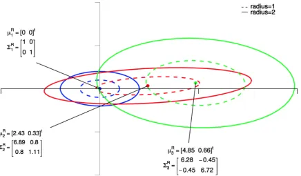
with unequal covariance matrices and original dimension p=6. Note that unlike the low-dimensional representation of [18], our Theorem 1 does not restrict the reduced dimension to be r=1.

5.2. Example

Consider the configuration N

(

µ₁,Σ₁

)

, N

(

µ₂,Σ₂

)

, and N

(

µ₃,Σ₃

)

, where

[

]

1= 0, 0, 0, 0, 0, 0 ,

µ

[

]

2= 1,1,1,1,1,1 ,

µ

[

]

3= 2, 2, 2, 2, 2, 2 ,

µ

1 2 3

1 0 0 0 0 0 2 1 1 1 1 1 2 1 0 1 1 1

0 1 0 0 0 0 1 2 1 1 1 1 1 2 0 1 1 1

0 0 1 0 0 0 1 1 2 1 1 1 0 0 7 0 0 0

, , and .

0 0 0 1 0 0 1 1 1 2 1 1 1 1 0 2 1 1

0 0 0 0 1 0 1 1 1 1 2 1 1 1 0 1 2 1

0 0 0 0 0 1 1 1 1 1 1 2 1 1 0 1 1 2

     

     

=  =  = 

     

     

Σ Σ Σ

We have rank

( )

M =2, and, thus, by Theorem 1, the six-dimensional multivariate normal densities can be compressed to the dimension q=2 without increasing the BPMC.

Using Theorem 1, we have that an optimal two-dimensional representation space is Col F

( )

, where

0.3800 0.3800 0.5272 0.3800 0.3800 0.3800 . 0.2358 0.2358 0.8497 0.2358 0.2358 0.2358

′

 

=  ₋ 

 

F (8)

(7)

We can also determine a one-dimensional representation of the three multivariate normal populations through application of the SVD described in Theorem 2 applied to the matrix M given in (7). A one-dimensional repre-sentation space is column one of the matrix F in (8), and the graphical representation of this configuration of univariate normal densities is depicted inFigure 2.

6. Four LDR Methods for Statistical Discrimination

[image:7.595.99.536.197.452.2] [image:7.595.89.540.477.708.2]

In this section, we present and describe the four LDR methods that we wish to compare and contrast in Sections 7 and 8.

Figure 1. The optimal two-dimensional representation for normal densities from the example in Section 5.2.

(8)

6.1. The SY Method

In Theorem 1, we assume the parameters µ_i and Σ_i, i=1,,m, are known, but in reality this assumption is rarely the case. In a sampling situation, we can replace the columns of the M matrix in (7) by their sample es-timators yielding

1 1 1 1 1 1

2 2 1 1 3 3 1 1 1 1 2 1 1

ˆ _| _| _| _| _| _| _,

m m m

− − − − − −

 

≡_ − −  − −  − _

M S x S x S x S x S x S x S S S S

provided n_i> p, i=1,,m. Our estimator Mˆ , along with Theorems 1 and 2, yields a LDR technique based on the selection of an r-dimensional hyperplane determined from a rank-r approximation to the full-rank matrix

ˆ

M.

Thus, using the SVD, we let Mˆ =UD V_p , where D_p≡diag

(

λ₁,,λ_p

)

, λ >j 0 are the singular values of

ˆ

M for j=1,,p, and let Fˆ =UD_p. Also, let

(

1 1

)

diag , , , 0 , , 0 r≡ λ  λr r+  p

D (9)

with λ_j≥λ_l for 1≤ < ≤j l p and 1≤ <r p. From Theorem 2, we have that M_r =UD V_r ′ is a rank-r ap-proximation of Mˆ , and a rank-r approximation to F is F_r =UD_r. Thus, F_r′ is our new r×p LDR matrix.

Provided

(

) (

)

1 1

p p

j j j r= +λ i=λ

 



∑

 is relatively small, Fr′ will yield an EPMC r

( )

such that

( )

EPMC p ≈EPMC r , and in certain population parameter configurations, we may have that

( )

EPMC r <EPMC p . We refer to our new LDR matrix as the SYLDR method.

6.2. The BE Method

A second LDR method presented by [14] is

(

) (

1

)

(

) (

1

)

(

) (

1

)

1 2 1 2 | | i j i j | | m 1 m m1 m

− −

−

− −

 

≡_ + − + − + − _

   

U Σ Σ µ µ Σ Σ µ µ Σ Σ µ µ

for 1≤ < ≤i j m, provided all multivariate normal population parameters are known. For the unknown parameter case, an estimator of U is then

(

) (

1

)

(

) (

1

)

(

) (

1

)

1 2 1 2 1 1

ˆ _| _| _| _| _.

i j i j m m m m

− −

−

− −

 

≡_ + − + − + − _

   

U S S x x S S x x S S x x (10)

The LDR matrix derived in [14], which we refer to as the BE matrix, was also obtained when we determined low-rank approximation to Uˆ by using the SVD. That is, let Uˆ =RD S_p ′ be the SVD of Uˆ, where

(

1

)

diag , , p ≡ λ  λp

D (11)

with λ_j≥λ_l for 1≤ < ≤j l p, and let Hˆ =RD_p. Define D_r as in (9) with λ_j ≥λ_l for 1≤ ≤j r. Then,

r ′ = 

U RD S is a rank-r approximation of Uˆ , and H =RD_r =R_r∈_{p r}_× is a rank-r approximation of Hˆ . Thus, the BE LDR matrix is H_r′, or, equivalently, R'r, where the

th

j eigenvector corresponds to the jth largest singular value and j=1,,r.

The BELDR approach is based on the rotated differences in the means. The LDR matrix (10) uses a type of pooled covariance matrix estimator for the precision matrices. However, the BE method does not incorporate all of the information contained in the different individual covariance matrices. Another disadvantage of the BE LDR approach is that it is limited to a reduced dimension that depends on the number of classes, m. For m=2,

BE allows one to reduce the data to only one dimension, regardless of the full-feature vector dimension. There-fore, one may lose some discriminatory information with the application of the BELDR method when the cova-riance matrices are considerably different.

6.3. Sliced Inverse Regression (SIR)

The next LDR method we consider is sliced inverse regression (SIR), which was proposed in [16]. Assuming all population parameters are known, we first define

1 m W ≡

∑

i= i m

Σ Σ as the within-group covariance matrix and

(

)(

)

1

m

B i= i i

m

′

≡

∑

−

Σ

µ µ µ µ

as the between-group covariance matrix, where

1 m

i i= m

≡

∑

(9)

population mean. As its criterion matrix, the SIRLDR method uses 2 2 1 1 , SIR B − − ≡

M Γ Σ Γ (12)

where Γ Σ≡ _B+Σ_W is the marginal covariance matrix of

x

. When population parameters must be estimated, an estimator of (12) is

1 2 1 2

ˆ ˆ ˆ _,

SIR B

− −

≡

M Γ S Γ (13)

where Γˆ ≡S_B+S_W with S_W and S_B given in (1) and (2), respectively. Let Mˆ_SIR =GD P_p ′ be the SVD of (13), and let Kˆ =Γˆ−12G_p, where G_p is composed of eigenvectors of (13) such that the th

j eigenvector of (13) corresponds to the th

j largest singular value of (13), j=1,,p. Then, _ˆ _ˆ 1 2

r Gr

−

=

K Γ is a rank-r ap-proximation of Kˆ, and the r×p SIRLDR matrix is Kˆ_r′, which is composed of the eigenvectors correspond-ing to the r largest singular values of K.

6.4. Sliced Average Variance Estimation (SAVE)

The last LDR method we consider is sliced average variance estimation (SAVE), which has been proposed in

[19]-[20]. The SAVE method uses the p×p criterion matrix *

(

12 2

)

2

1

m

SAVE i p i m

− − =

≡

∑

−

M I Γ Σ Γ , where

B W

≡ +

Γ Σ Σ . We use a form of SAVE given in [21], which is

(

12 12

)

2 12 12

,

SAVE B

− − − −

≡ +

M Γ Σ Γ Γ Σ ΓΓ (14)

where

(

) (

1

)

1 m

i W i W

i m

− =

≡

∑

− −

Γ

Σ Σ Σ Γ Σ Σ . An estimator of M_SAVE is

(

12 12

)

2 12 12 ˆ

ˆ ˆ ˆ ˆ ˆ _,

SAVE B

− − − −

≡ +

M Γ S Γ Γ S_ΓΓ (15)

where,

(

) (

1

)

ˆ 1

ˆ m

i W i W

i m

− =

≡

∑

− −

S_Γ S S Γ S S with S_W and S_B given in (1) and (2), respectively. Next, let

ˆ

SAVE = p ′

M BD Q be the SVD of (15), and let Lˆ=Γˆ−12B_p, where B_p is composed of the eigenvectors of (15) such that the th

j column of B_p corresponds to the th

j of (15) with the th

j largest singular value,

1, ,

j=  p. Then, _ˆ _ˆ 1 2

r r

−

=

L Γ B is a rank-r approximation of Lˆ, and, thus, the r×p SAVELDR matrix is

ˆ

r′

L . An alternative representation of the r-dimensional SAVELDR matrix is B_r, which is composed of the ei-genvectors corresponding to the r largest singular values of B.

7. A Monte Carlo Comparison of Four LDR Methods for Statistical Classification

Here, we compare our new SYLDR method derived above to the BE, SIR, and SAVELDR methods. Specifically, we evaluate the classification efficacy in terms of the EPMC for the SY, BE, SIR, and SAVELDR methods using Monte Carlo simulations for five different configurations of multivariate normal populations with p=10. We have generated 10,000 training-sample and test datasets from the appropriate multivariate normal distributions for each parameter configuration. The test data were assigned to either population class Π₁ or Π₂ when

2

m= or Π₁, Π₂, or Π₃ when m=3 using the sample QDF corresponding to (4). We have applied the four competing LDR matrices F_r′, H_r′, K_r′, and L_r′ and calculated the EPMCs for the full-dimensional QDF

and for the four reduced-dimensional QDFs by averaging the estimated conditional error rate over all training samples. We examined the effect of the training-sample sizes on the four LDR methods using sample sizes

( )

2.5

i

n = p and ni =5p, i=1, 2 or i=1, 2, 3.

For the SY and SAVELDR approaches, we reduce the dimension to r=1, 2, 3. In general, for m populations, we remark that the BE LDR method can reduce the feature vector to at most the dimension r=m m

(

−1 2

)

(10)

populations m.

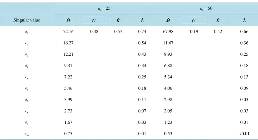
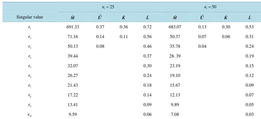
The five Monte Carlo simulations were generated using the programming language R. Table 1 gives a description of the number of populations and the theoretically optimal rank of the four LDR indices for each configuration. InFigures 3-7, we display the corresponding EPMCs of the four competing LDR methods for the various population configurations and values of n_i and r, where i=1,,m. The estimated standard error of all EPMCs in the following tables was less than 0.001. For each configuration, we also calculated ˆM, Uˆ , ˆK, and Lˆ along with their respective singular values using the SVD. These singular values contain information concerning the amount of discriminatory information available in each reduced dimension. In the subsequent subsections, we use the following notation: EPMC_r

( )

SY , EPMC_r

( )

BE , EPMC_r

(

SIR

)

, and EPMC_r

(

SAVE

)

denote the estimated EPMCs for the SY, BE, SIR, and SAVE LDR methods, respectively, for each of the appropriate reduced dimensions.

7.1. Configuration 1: m = 2 with Moderately Different Covariance Matrices

The first population configuration we examined was composed of two multivariate normal populations

(

, 1

)

p

N 0Σ and Np

(

µ₂,Σ₂

)

, where p=10,

[

]

1

=

0, 0, 0, 0, 0, 0, 0, 0, 0, 0 ,

′

µ

[

]

2= 5,5,5,5,5,5,5,5,5,5 ,′

[image:10.595.88.540.362.690.2]

µ

Table 1. A description of Monte Carlo simulation parametric configurations and singular values in Section 2 with unequal covariance matrices and p=10.

Rank

Configuration Means m M U K L

1 Moderately separated unequal means 2 3 1 1 2

2 Relatively close unequal means 3 2 1 1 2

5 Close unequal means 2 4 3 2 4

(a) (b)

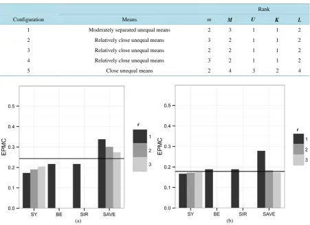
Figure 3. Simulation results from Section 7.1. The horizontal bar in each graph represents the EPMC10. (a) ni=25; (b) 50

i

(11)

(a) (b)

Figure 4. Simulation results from Configuration 2. The horizontal bar in each graph represents the EPMC₁₀ with no dimension reduction. (a) ni=25; (b) ni=50.

(a) (b)

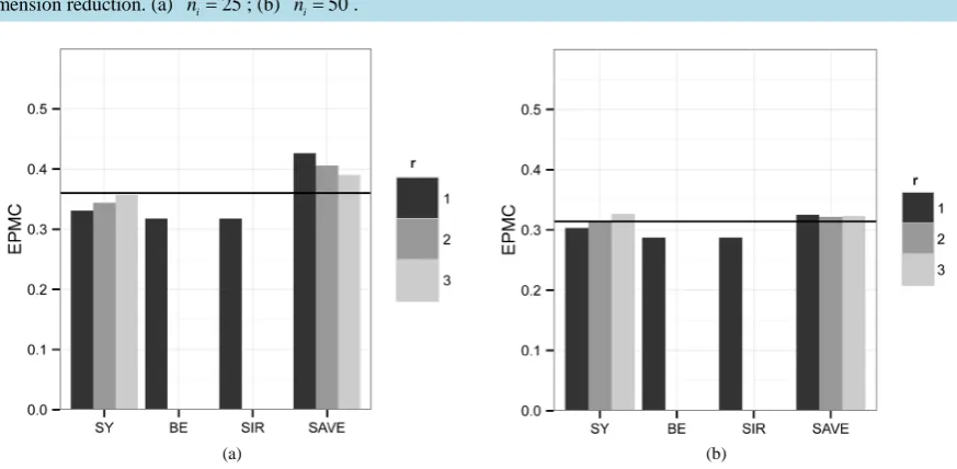
Figure 5.Simulation results from Section 7.3. The horizontal bar in each graph represents the EPMC10. (a) ni=25; (b) 50

i

n = .

1

10.00 4.00 5.00 4.00 3.00 4.00 4.00 5.00 4.00 3.00

4.00 10.00 5.00 2.00 4.00 3.00 3.00 5.00 4.00 3.00

5.00 5.00 10.00 5.00 5.00 3.00 4.00 4.00 4.00 4.00

4.00 2.00 5.00 10.00 3.00 4.00 2.00 3.00 4.00 3.00

3.00 4.00 5.00 3.00 10.00 3.00 4.00 5.00

=

Σ 3.00 3.00

4.00 3.00 3.00 4.00 3.00 12.00 3.00 4.00 4.00 4.00

4.00 3.00 4.00 2.00 4.00 3.00 14.00 2.00 2.00 2.00

5.00 5.00 4.00 3.00 5.00 4.00 2.00 12.00 0.50 0.50

4.00 4.00 4.00 4.00 3.00 4.00 2.00 0.50 14.00 1.00

3.00 3.00 4.00 3.00 3.00 4.00

− −

,

2.00 0.50 1.00 11.00

 

 

 − − 

 

[image:11.595.72.539.79.274.2] [image:11.595.96.533.298.512.2]

(12)

(a) (b)

Figure 6. Simulation results from Configuration 4. The horizontal bar in each graph represents the EPMC₁₀ with no dimension reduction. (a) n_i=25; (b) n_i=50.

[image:12.595.95.535.77.279.2]

(a) (b)

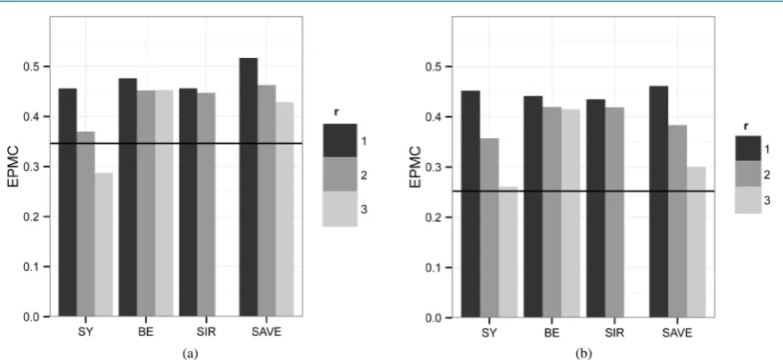
Figure 7. Simulation results from Section 7.5. The horizontal bar in each graph represents the EPMC10. (a) ni=25; (b) 50

i

n = .

2

16.00 10.00 11.00 10.00 9.00 10.00 10.00 11.00 10.00 9.00

10.00 16.00 11.00 8.00 10.00 9.00 9.00 11.00 10.00 9.00

11.00 11.00 16.00 11.00 11.00 9.00 10.00 10.00 10.00 10.00

10.00 8.00 11.00 16.00 9.00 10.00 8.00 9.00 10.00 9.00

9.00 10.00

=

Σ 11.00 9.00 16.00 9.00 10.00 11.00 9.00 9.00

10.00 9.00 9.00 10.00 9.00 18.00 9.00 10.00 10.00 10.00

10.00 9.00 10.00 8.00 10.00 9.00 20.00 8.00 8.00 8.00

11.00 11.00 10.00 9.00 11.00 10.00 8.00 22.00 9.50 9.50

10.00 10.00 10.00 10.00 9.00 10.0

.

0 8.00 9.50 24.00 9.00

9.00 9.00 10.00 9.00 9.00 10.00 8.00 9.50 9.00 21.00

 

 

[image:12.595.98.538.314.518.2]

(13)

Here, rank

(

Σ₂−Σ₁

)

=1, which implies rank

( )

M =2 because

(

1 1

)

(

)

2 2 1 1 span 2 1

− ₋ − _∉ ₋

Σ µ Σ µ Σ Σ . The

singular values of Mˆ in Table 2 indicate that most of the classificatory information can be captured when 1

r= , because the subsequent singular values are small relative to the first. Also, the BELDR technique loses classificatory information from pooling the acutely dissimilar pair of covariance matrices.

When ni =25, the EPMC was reduced by the SY, BE, and SIRLDR methods but not for the SAVE LDR

method. This effect occurred because the training-sample size ni =25, i=1, 2, are small relative to the full-

feature dimensionality p=10, and, therefore, insufficient data were available to accurately estimate the

(

3

)

p p+ total population parameters. Thus, by reducing the full-feature dimension p=10 to dimension 10

r , we considerably increased the ratio of the training-sample size relative to the original new dimension so that n r_i n p_i to n r_i , where rp. Thus, we achieved improved parameter estimates in the r-

dimensional subspaces. Not surprisingly, for ni =25, i=1, 2, we found that EPMC10−EPMC SY1

( )

≈0.06

and for ni =50, EPMC10−EPMC SY1

( )

≈0.01, which demonstrated the advantage of employing LDR in the classification process, and, more specifically, demonstrated the value of the SYLDR method. Additionally, as n_i increased, the EPMC_r

( )

⋅ approached EPMC_p

( )

⋅ for all four LDR methods as r increased.

In addition, the SIRLDR method did not utilize discriminatory information contained in the differences of the covariance matrices when ni =25, i=1, 2. However, for ni =50, i=1, 2, all four LDR methods yielded essentially the same EPMC, except for SAVE when r=1.

7.2. Configuration 2: m = 3 with Two Similar Covariance Matrices and One Spherical

Covariance Matrix

The second Monte Carlo simulation used a configuration with the three multivariate normal populations

(

1, 1

)

p

N µ Σ , Np

(

µ₂,Σ₂

)

, and Np

(

µ3,Σ3

)

where p=10,

[

]

1= 0, 0, 0, 0, 0, 0, 0, 0, 0, 0 ,′

µ

[

]

2 = 1, 1, 1, 1, 1, 1, 1, 1, 1, 1 ,′

µ

[

]

3 = 2, 2, 2, 2, 2, 2, 2, 2, 2, 2 ,′

[image:13.595.87.538.474.719.2]

µ

Table 2.Summary of singular values for the four competing LDR methods for Configuration 1. 25

i

n= n_i=50

Singular value _Mˆ _Uˆ _Kˆ _Lˆ _Mˆ _Uˆ _Kˆ _Lˆ

1

e 72.16 0.38 0.57 0.74 67.98 0.19 0.52 0.66

2

e 16.27 0.54 11.67 0.36

3

e 12.21 0.43 8.93 0.25

4

e 9.31 0.34 6.88 0.18

5

e 7.22 0.25 5.34 0.13

6

e 5.46 0.18 4.06 0.09

7

e 3.99 0.11 2.98 0.05

8

e 2.73 0.07 2.05 0.03

9

e 1.67 0.03 1.23 0.01

10

(14)

1

1.00 0.00 0.00 0.00 0.00 0.00 0.00 0.00 0.00 0.00

0.00 1.00 0.00 0.00 0.00 0.00 0.00 0.00 0.00 0.00

0.00 0.00 1.00 0.00 0.00 0.00 0.00 0.00 0.00 0.00

0.00 0.00 0.00 1.00 0.00 0.00 0.00 0.00 0.00 0.00

0.00 0.00 0.00 0.00 1.00 0.00 0.00 0.00 0.00 0

=

Σ .00

0.00 0.00 0.00 0.00 0.00 1.00 0.00 0.00 0.00 0.00

0.00 0.00 0.00 0.00 0.00 0.00 1.00 0.00 0.00 0.00

0.00 0.00 0.00 0.00 0.00 0.00 0.00 1.00 0.00 0.00

0.00 0.00 0.00 0.00 0.00 0.00 0.00 0.00 1.00 0.00

0.00 0.00 0.00 0.00 0.00 0.00 0.00 0.00 0.00 1 ,

.00

 

 

 

2

2.00 1.00 1.00 1.00 1.00 1.00 1.00 1.00 1.00 1.00

1.00 2.00 1.00 1.00 1.00 1.00 1.00 1.00 1.00 1.00

1.00 1.00 2.00 1.00 1.00 1.00 1.00 1.00 1.00 1.00

1.00 1.00 1.00 2.00 1.00 1.00 1.00 1.00 1.00 1.00

1.00 1.00 1.00 1.00 2.00 1.00 1.00 1.00 1.00 1

=

Σ .00

1.00 1.00 1.00 1.00 1.00 2.00 1.00 1.00 1.00 1.00

1.00 1.00 1.00 1.00 1.00 1.00 2.00 1.00 1.00 1.00

1.00 1.00 1.00 1.00 1.00 1.00 1.00 2.00 1.00 1.00

1.00 1.00 1.00 1.00 1.00 1.00 1.00 1.00 2.00 1.00

1.00 1.00 1.00 1.00 1.00 1.00 1.00 1.00 1.00 2 ,

.00

 

 

 

and

3

2.00 1.00 0.00 1.00 1.00 1.00 1.00 1.00 1.00 1.00

1.00 2.00 0.00 1.00 1.00 1.00 1.00 1.00 1.00 1.00

0.00 0.00 10.00 0.00 0.00 0.00 0.00 0.00 0.00 0.00

1.00 1.00 0.00 2.00 1.00 1.00 1.00 1.00 1.00 1.00

1.00 1.00 0.00 1.00 2.00 1.00 1.00 1.00 1.00

=

Σ 1.00

1.00 1.00 0.00 1.00 1.00 2.00 1.00 1.00 1.00 1.00

1.00 1.00 0.00 1.00 1.00 1.00 2.00 1.00 1.00 1.00

1.00 1.00 0.00 1.00 1.00 1.00 1.00 2.00 1.00 1.00

1.00 1.00 0.00 1.00 1.00 1.00 1.00 1.00 2.00 1.00

1.00 1.00 0.00 1.00 1.00 1.00 1.00 1.00 1.00

.

2.00

 

 

 

In this configuration, the population means are unequal but relatively close. Moreover, Σ₂ and Σ₃ are un-equal but notably more similar to one another than to Σ₁. However, the variance of the third feature in Π₃ is significantly greater than the population variances of the third feature for either Π₁ or Π₂.

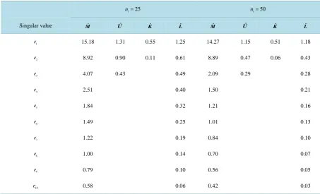
As a result of markedly different covariance matrices, the BE and SIRLDR methods are not ideal because both methods aggregated the sample covariance matrices. The SYLDR method, however, attempts to estimate each individual covariance matrix for all three populations, and uses this information that yielded SY as the su-perior LDR procedure.Table 3 gives the singular values of each of the LDR methords considered here.

For the larger sample-size scenario, ni =50, i=1, 2, the SAVE LDR was more competitive with SY than

either BE or SIR when r>1. However, the SYLDR remained the preferred LDR method. In Figure 4, we add-ed noise to the SY method when we used r>2, and, we eliminated essential discriminatory information for the

(15)

[image:15.595.84.538.100.375.2]

Table 3. Summary of singular values for the four competing LDR methods applied to Configuration 2. 25

i

n = ni=50

Singular value Mˆ Uˆ Kˆ Lˆ Mˆ Uˆ Kˆ Lˆ

1

e 15.18 1.31 0.55 1.25 14.27 1.15 0.51 1.18

2

e 8.92 0.90 0.11 0.61 8.89 0.47 0.06 0.43

3

e 4.07 0.43 0.49 2.09 0.29 0.28

4

e 2.51 0.40 1.50 0.21

5

e 1.84 0.32 1.21 0.16

6

e 1.49 0.25 1.01 0.13

7

e 1.22 0.19 0.84 0.10

8

e 1.00 0.14 0.70 0.07

9

e 0.79 0.10 0.56 0.05

10

e 0.58 0.06 0.42 0.03

that _EPMC₁₀

( )

SY −EPMC₂

( )

SY _≈0.10 for ni = 50 and EPMC10

( )

SY −EPMC2

( )

SY ≈0.15 for ni = 25,

1, 2, 3

i= . This significant reduction from EPMC₁₀ demonstrated a significant benefit of dimension reduction in general and the SYLDR in particular.

7.3. Configuration 3: m = 2 with Relatively Close Means and Different But Similar

Covariance Matrices

In this configuration, we have Np

(

µ₁,Σ₁

)

and Np

(

µ2,Σ2

)

with p=10,

[

]

1 = 0, 0, 0, 0, 0, 0, 0, 0, 0, 0 ,′

µ

[

]

2= 2, 2, 2, 2, 2, 2, 2, 2, 2, 2 ,′

µ

1

10.00 4.00 5.00 4.00 3.00 4.00 4.00 5.00 4.00 3.00

4.00 10.00 5.00 2.00 4.00 3.00 3.00 5.00 4.00 3.00

5.00 5.00 10.00 5.00 5.00 3.00 4.00 4.00 4.00 4.00

4.00 2.00 5.00 10.00 3.00 4.00 2.00 3.00 4.00 3.00

3.00 4.00 5.00 3.00 12.00 3.00 4.00 5.00

=

Σ 3.00 3.00

4.00 3.00 3.00 4.00 3.00 9.00 3.00 4.00 4.00 4.00

4.00 3.00 4.00 2.00 4.00 3.00 14.00 2.00 2.00 2.00

5.00 5.00 4.00 3.00 5.00 4.00 2.00 12.00 1.00 0.50

4.00 4.00 4.00 4.00 3.00 4.00 2.00 1.00 14.00 1.00

3.00 3.00 4.00 3.00 3.00 4.00 2.0

− −

,

0 0.50 1.00 11.00

 

 

 − − 

 

(16)

2

8.00 2.00 3.00 4.00 1.00 2.00 2.00 3.00 2.00 1.00

2.00 8.00 3.00 2.00 2.00 1.00 1.00 3.00 2.00 1.00

3.00 3.00 8.00 5.00 3.00 1.00 2.00 2.00 2.00 2.00

4.00 2.00 5.00 10.00 3.00 4.00 2.00 3.00 4.00 3.00

1.00 2.00 3.00 3.00 10.00 1.00 2.00 3.00 1.0

=

Σ 0 1.00

2.00 1.00 1.00 4.00 1.00 7.00 1.00 2.00 2.00 2.00

2.00 1.00 2.00 2.00 2.00 1.00 12.00 0.00 0.00 0.00

3.00 3.00 2.00 3.00 3.00 2.00 0.00 10.00 1.00 2.50

2.00 2.00 2.00 4.00 1.00 2.00 0.00 1.00 12.00 3.00

1.00 1.00 2.00 3.00 1.00 2.00 0.00

− −

.

2.50 3.00 9.00

 

 

 − − 

 

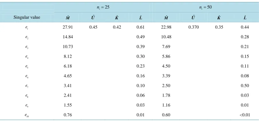
As in Configuration 1, we have that rank

(

Σ₂−Σ₁

)

=1, and, hence, rank

( )

M =2. In Configuration 3, the

BE and SIR LDR methods outperformed the SY and SAVE LDR methods because of the similarity in the covariance matrices. This phenomenon occurred because both LDR methods aggregated the sample covariance matrices, which resulted in less-variable covariance matrix estimators and, therefore, smaller values of

( )

1

EPMC BE and EPMC SIR₁

(

)

. FromTable 4, we see that the first singular value for ˆM was considerably less predominant than the first singular value for ˆM in Configuration 1. This result explained the inferiority of the SY method for this configuration, regardless of the chosen n_i, i=1, 2.

For r=1, we have that _EPMC₁₀−EPMC SIR₁

(

)

_{ } ≈ EPMC₁₀−EPMC BE₁

( )

_≈0.04 for ni =25 and

(

)

( )

10 1 10 1 0.06

EPMC −EPMC SIR ≈ EPMC −EPMC BE ≈

   

    for ni =50. Again, we exemplify the value of LDR as a classification tool. In this configuration, not only was EPMC₁₀ considerably reduced as n_i in-creased, but the difference between _EPMC₁₀−EPMC BE₁

( )

_ and _EPMC₁₀−EPMC SIR₁

(

)

_ decreased as well. This example demonstrated the fact that the SY method is not a uniformly superior LDR approach even when covariance matrices are unequal. However, EPMC SY₁

( )

was not much greater than either EPMC BE₁

( )

or EPMC SIR₁

(

)

. Here, SAVE is not as competitive as the three other LDR methods because it does not use all the information in the difference of the covariance matrices and means to obtain a better information-preserving subspace.

7.4. Configuration 4: m = 3 with Two Similar Covariance Matrices Except for the First Two

Dimensions

[image:16.595.86.539.512.723.2]

In this situation, we have three multivariate normal populations: Np

(

µ₁,Σ₁

)

, Np

(

µ2,Σ2

)

, and Np

(

µ3,Σ3

)

,

Table 4. Summary of singular values for the four competing LDR methods for Configuration 3. 25

i

n = ni=50

Singular value _Mˆ _Uˆ _Kˆ _Lˆ _Mˆ _Uˆ _Kˆ _Lˆ

1

e 27.91 0.45 0.42 0.61 22.98 0.370 0.35 0.44

2

e 14.84 0.49 10.48 0.28

3

e 10.73 0.39 7.69 0.21

4

e 8.12 0.30 5.86 0.15

5

e 6.18 0.23 4.50 0.11

6

e 4.65 0.16 3.39 0.08

7

e 3.41 0.10 2.50 0.50

8

e 2.41 0.06 1.78 0.03

9

e 1.55 0.03 1.16 0.01

10

(17)

where p=10,

[

]

1= 0, 0, 0, 0, 0, 0, 0, 0, 0, 0 ,′

µ

[

]

2= 1, 0, 1, 0, 1, 0, 1, 0, 1, 0 ,′

µ

[

]

3= − − − − − − − − − −1, 1, 1, 1, 1, 1, 1, 1, 1, 1 ,′

µ

1

2.00 0.80 1.00 0.80 0.60 0.80 0.80 1.00 0.80 0.60

0.80 2.00 1.00 0.40 0.80 0.60 0.60 1.00 0.80 0.60

1.00 1.00 2.00 1.00 1.00 0.60 0.80 0.80 0.80 0.80

0.80 0.40 1.00 2.00 0.60 0.80 0.40 0.60 0.80 0.60

0.60 0.80 1.00 0.60 2.00 0.60 0.80 1.00 0.60 0

=

Σ .60

0.80 0.60 0.60 0.80 0.60 2.40 0.60 0.80 0.80 0.80

0.80 0.60 0.80 0.40 0.80 0.60 2.80 0.40 0.40 0.40

1.00 1.00 0.80 0.60 1.00 0.80 0.40 2.40 0.10 0.10

0.80 0.80 0.80 0.80 0.60 0.80 0.40 0.10 2.80 0.20

0.60 0.60 0.80 0.60 0.60 0.80 0.40 0.10

− − − − − , 0.20 2.20                              −    2

20.00 0.80 1.00 0.80 0.60 0.80 0.80 1.00 0.80 0.60

0.80 40.00 1.00 0.40 0.80 0.60 0.60 1.00 0.80 0.60

1.00 1.00 2.00 1.00 1.00 0.60 0.80 0.80 0.80 0.80

0.80 0.40 1.00 2.00 0.60 0.80 0.40 0.60 0.80 0.60

0.60 0.80 1.00 0.60 2.00 0.60 0.80 1.00 0.6

=

Σ 0 0.60

0.80 0.60 0.60 0.80 0.60 2.40 0.60 0.80 0.80 0.80

0.80 0.60 0.80 0.40 0.80 0.60 2.80 0.40 0.40 0.40

1.00 1.00 0.80 0.60 1.00 0.80 0.40 2.40 0.10 0.10

0.80 0.80 0.80 0.80 0.60 0.80 0.40 0.10 2.80 0.20

0.60 0.60 0.80 0.60 0.60 0.80 0.40 0.

− −

−

,

10 0.20 2.20

                             −    and 3

35.00 0.80 1.00 0.80 0.60 0.80 0.80 1.00 0.80 0.60

0.80 40.00 1.00 0.40 0.80 0.60 0.60 1.00 0.80 0.60

1.00 1.00 2.00 1.00 1.00 0.60 0.80 0.80 0.80 0.80

0.80 0.40 1.00 2.00 0.60 0.80 0.40 0.60 0.80 0.60

0.60 0.80 1.00 0.60 2.00 0.60 0.80 1.00 0.6

=

Σ 0 0.60

0.80 0.60 0.60 0.80 0.60 2.40 0.60 0.80 0.80 0.80

0.80 0.60 0.80 0.40 0.80 0.60 2.80 0.40 0.40 0.40

1.00 1.00 0.80 0.60 1.00 0.80 0.40 2.40 0.10 0.10

0.80 0.80 0.80 0.80 0.60 0.80 0.40 0.10 2.80 0.20

0.60 0.60 0.80 0.60 0.60 0.80 0.40 0.

− −

−

.

10 0.20 2.20

                             −   

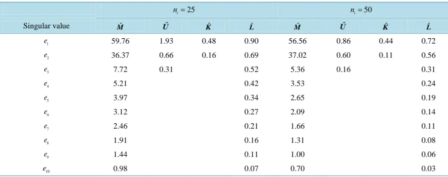
For the fourth configuration, the covariance matrices are considerably different from one another, which ben-efits both the SY and SAVELDR methods. Specifically, the SYLDR procedure uses information contained in the unequal covariance matrices to determine classificatory information contained in S_j −S₁ and in S x−_j1 _j−S x₁−1 ₁,

2, 3

(18)

de-creased as r increased. For the SY method, we have rank

( )

M =4, which clarifies the reason that EPMC_r

( )

SY and r were inversely related. As one can see in Table 5, the first three singular values of Mˆ were relatively large. However, the pooling of the sample covariance matrices used in BE and SIR tended to obscure classifica-tory information in the sample covariance matrices. The only improvement from the full dimension we found for the values of r and n_i considered here was the SY method when r=3 for ni =25, i=1, 2, 3. Specifically,

we have that _EPMC₁₀−EPMC₃

( )

SY _≈0.05 when ni =25, although EPMC10−EPMC3

( )

SY ≈ −0.01 when ni =50, i=1, 2, 3.

This population configuration illustrated the fact that we cannot always choose r=1 and expect to see a re-duction in EPMC_p. However, we can often reduce the EPMC_p if we use both a judicious choice of r and an appropriate LDR method.

7.5. Configuration 5: m = 3 with Diverse Population Covariance Matrices

In Configuration 5, we have three multivariate normal populations: Np

(

µ₁,Σ₁

)

, Np

(

µ2,Σ2

)

, and Np

(

µ3,Σ3

)

,

where p=10,

[

]

1= 0, 0, 0, 0, 0, 0, 0, 0, 0, 0 ,′

µ

[

]

2 = 4.43, 4.43, 4.43, 4.43, 4.43, 4.43, 4.43, 4.43, 4.43, 4.43 ,′

µ

[

]

3= 8,8,8,8,8,8,8,8,8,8 ,′

µ

with

1

15.01 0.81 1.25 1.13 2.10 2.30 2.43 3.30 0.87 1.11

0.81 26.10 1.51 0.74 0.89 4.35 1.25 1.85 0.50 0.39

1.25 1.51 24.55 5.57 3.96 1.62 0.27 0.49 5.97 0.87

1.13 0.74 5.57 29.36 3.58 0.89 2.21 3.71 0.52 2.19

2.10 0.89 3.96 3

− − − − −

− − −

− − − − − − −

− −

=

Σ .58 20.17 6.05 5.20 2.22 0.80 2.69

2.30 4.35 1.62 0.89 6.05 40.18 5.18 3.83 1.94 0.51

2.43 1.25 0.27 2.21 5.20 5.18 17.93 0.17 3.09 0.49

3.30 1.85 0.49 3.71 2.22 3.83 0.17 26.05 0.54 3.34

0.87 0.50 5.97 0.52 0.80 1.94 3.09

− − −

− − − − −

− − − −

− − − − − −

,

0.54 16.30 1.04

1.11 0.39 0.87 2.19 2.69 0.51 0.49 3.34 1.04 26.84

 

 

 ₋ ₋ 

 

− − − − − 

[image:18.595.88.537.541.719.2]

 

Table 5. Summary of singular values for the four competing LDR methods for Configuration 4. 25

i

n = n_i=50

Singular value _Mˆ _Uˆ _Kˆ _Lˆ _Mˆ _Uˆ _Kˆ _Lˆ 1

e 59.76 1.93 0.48 0.90 56.56 0.86 0.44 0.72

2

e 36.37 0.66 0.16 0.69 37.02 0.60 0.11 0.56

3

e 7.72 0.31 0.52 5.36 0.16 0.31

4

e 5.21 0.42 3.53 0.24

5

e 3.97 0.34 2.65 0.19

6

e 3.12 0.27 2.09 0.14

7

e 2.46 0.21 1.66 0.11

8

e 1.91 0.16 1.31 0.08

9

e 1.44 0.11 1.00 0.06

10