Adaptive Quantum Inspired Genetic Algorithm for Combinatorial Optimization Problems

Adaptive Quantum Inspired Genetic Algorithm for

Combinatorial Optimization Problems

Jyoti Chaturvedi

D.E.I. (Deemed University), Dayalbagh, Agra, U.P.

India

ABSTRACT

The development in the field of quantum computing gives us a significant edge over classical computing in terms of time and efficiency. This is particularly useful for NP-hard problems such as graph layout problems. Since many real world problems are effectively solved by genetic algorithm (GA) and the performance of GA highly depends upon the setting of its parameters, therefore this paper focuses on a Quantum Inspired Genetic Algorithm (QIGA) and develops and evaluates adaptive strategies for the same. QIGA adapts ideas of Q-bits, superposition of Q-bits from quantum computing. The effectiveness and the applicability of adaptive QIGA is demonstrated by experimental results on the benchmark Knapsack, Maxcut and Onemax combinatorial optimization problems. The results show that adaptive QIGA is superior to QIGAs.

Keywords

Quantum inspired genetic algorithm, Parameter control, adaptive QIGA.

1.

INTRODUCTION

To find the solution of combinatorial optimization problems randomness in the search gives high probability to search a good solution. Stochastic optimization is the general class of algorithms which employ some degree of randomness to find optimal (or near optimal) solutions to hard problems. The primary subfield of the stochastic search is Meta-heuristics [1]. Meta-heuristics approaches can be broadly categorized into two major classes: single solution search algorithms and population based search algorithms (e.g. evolutionary algorithm, swarm optimization techniques, ant colony optimization etc.). In Meta-heuristics, population based search methods (e.g. genetic algorithms, evolutionary strategies etc.) are very efficient as they keep around a sample of candidate solutions rather than a single candidate solution and find the optimal solution in less time [1]. This paper focuses on Quantum Inspired Genetic Algorithm. QIGA is a probabilistic population based algorithm as it works on the principles of quantum computing. It includes additional degree of randomness which helps in preserve diversity in the algorithm.

The efficiency of the algorithm highly depends upon its parameter setting. If the parameters are set to their optimal values, then algorithm may converge to the optimal solutions quickly. The setting of parameters is extremely hard task as they are problem specific and interdependent [2-6]. Thus, for a long time scientists and researchers are concentrating on finding techniques for effective use and change of parameters

involved in the search methods to improve their performance [7-11].

In this paper, an adaptation technique is devised to update the parameters of Quantum Inspired Genetic algorithm (QIGA) that aims at biasing the distribution towards appropriate regions of the search space while maintaining sufficient diversity among individuals in order to widen the search space.

2.

QUANTUM INSPIRED GENETIC

ALGORITHM (QIGA)

In QIGA some of the features of quantum computing are implemented with the concepts of genetic algorithm [12-13]. Here QIGA, the representation of the population individual is inspired by the concept of Q-bit in quantum computing. Before start discussing about Q-bit individuals, the concept of Q-bits is first introduced in Quantum Computing by us. Q-bit is the basic building block of quantum computing [14]. Q-bit can be represented in a two dimensional state space. The basis states of this space are generally taken as orthonormal states [15]. QIGA uses a new representation for the probabilistic representation of an individual that is based on the concept of Q-bits. A Q-bit individual is a string of m Q-bits, which is defined below.

𝛂𝟏

𝛃𝟏

𝛂𝟐

𝛃 𝟐

𝛂𝟑

𝛃𝟑

⋯ ⋯

𝛂𝐦

𝛃𝐦

Here αi and βi are the probability of getting 0 and 1 respectively at position i. Also |αi|2+ |βi|2=1, for i=1,2,...m. A population of n Q-bit individuals, Q(t)={qt1,qt2,…,qtn}, at generation t, with a Q-bit individual qtj is defined as [12]

𝐪𝐣𝐭=

𝛂𝐣𝟏𝐭

𝛃𝐣𝟏𝐭

𝛂𝐣𝟐𝐭

𝛃𝐣𝟐𝐭

𝛂𝐣𝟑𝐭

𝛃𝐣𝟑𝐭

⋯ ⋯

𝛂𝐣𝐦𝐭

𝛃𝐣𝐦𝐭

, j=1,2,…m.

where m is the number of Q-bits, i.e., the string length of the Q-bit individual.

3.

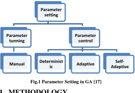
TAXONOMY OF ADAPTATION

Fig.1 Parameter Setting in GA [17]

4.

METHODOLOGY

Present section presents components of QIGA, and proposed adaptive QIGA.

4.1

Representation of Individual

There are two types of individuals (chromosomes) that are used in the proposed QIGA [4]:

1. Probabilistic Quantum chromosome 2. Binary solution chromosome

A quantum chromosome is one dimensional array containing real numbers. This chromosome is divided in two halves. First half contains the amplitude, square of which gives the probability of getting one at the corresponding index position. The other half contains the standard deviations for adapting the mutation step size based on normal distribution corresponding to index positions of first half. Thus the quantum chromosome is double in size of the solution chromosome of the problem.

Binary solution chromosome or simply solution chromosome of the problem is a one dimensional array that contains 0 or 1 in it according to the probability of one in the quantum chromosome at the corresponding index position. 1 or 0 represents inclusion or exclusion respectively of the index in the solution (whatever the index position represents). An example of solution chromosome is presented in figure 5 in which item number 2, 3 and 29 are included among 30 items.

4.2

Operators used in QIGA

The components that are used in adaptive QIGA are as follows:

1) Fitness function: To evaluate the fitness of the given solution chromosome there is a fitness function that is used and it is problem dependent [13] (generally taken as objective function of the problem).

2) Selection procedure: Recombination and mutation is applied on some selective quantum individuals of the population. For the selection of these individuals there are many procedures [13]. In the present paper group selection is used that is described by the following example. Let the population be divided into three equal groups according to the fitness of the individuals (i.e. best, medium and least fit). Let us select 50% from best fit individuals, 30% from medium fit individuals and 20% from least fit individuals to accomplish selection [13].

3) Recombination: There are two recombination (crossover) operators used for quantum individuals in this work [13].

a). Multi point crossover, b). Uniform crossover

4) Mutation: The mutation strategy described here is inspired by [7]. To mutate a quantum individual a random number is

drawn from normal distribution with mean 0 and standard deviation σ and then this random number is added or subtracted to the values at all positions of first half of the quantum individual Q according to the success of the solution chromosome as follows:

qi‟= qi ± σi‟* N(0,1), i=1,2,3…m

where qi‟ is the new value of quantum individual at position i, qi is the old value of quantum chromosome at position i, σi‟ is the standard deviation used for quantum chromosome value at index i, m is the length of solution chromosome and N(0,1) gives the random number from the normal distribution with mean 0 and standard deviation1 (similarly N(0,σ) gives normal distribution with mean 0 an standard deviation 1 by multiplying it with σ).

In this procedure standard deviations σi also mutate itself as follows:

σi‟ = c*σi

Where c = (1-qi) or qi and σi is the previous value of standard deviation. Here overall mutation scale is governed by the value of σ, which is why it is commonly referred to as step size.

Index1 Index 2 Index 3 … Index 28 Index29 Index 30

Fig. 2. Solution Chromosome

4.3

Proposed Adaptations on QIGA

The motivation of adaptation in various parameters is that to obtain best overall performance of QIGA on complex problems [18]. With the probabilistic representation of quantum individuals as described previously, adaptations applied to the parameters of QIGA are described below. Crossover adaptation: The adaptive crossover operator used here is the “selective crossover” that uses a number of crossovers and among them only one at a time is selected for pair of individuals. For the application of this adaptive crossover an extra crossover bit (crbit) is used in each population individuals. The value of this bit is decided according to the progress in the algorithm due to given crossover and this crbit then decides which crossover would be used in the next iteration [19]. Pseudo code for the “selective crossover” is given below.

Parameter setting

Parameter tunning

Manual

Parameter control

Determinist

ic Adaptive

Self-Adaptive

Choose i and j as parents crossover begin if(crbit(i)==crbit(j)==1)

use two point crossover to produce child if(success)

crbit(child)=crbit(i) end

end

if(crbit(i)==crbit(j)==0)

use uniform crossover to produce child if(success)

crbit(child)=crbit(i) end

end

if(crbit(i)~=crbit(j)) if(rand(0,2)<1)

use two point crossover to produce child. else

use uniform crossover to produce child end

If(success)

crbit(child)=choose between crbit(i) and crbit(j) end

end

Crossover rate adaptation: The probability of crossover Pc is adapted according to the fitness values of the individuals. The adaptation of pc allows the individuals having fitness values i.e.over- average to maintain their genetic material, while forcing the individuals with sub- average fitness values to disrupt [11].

If (fcmax>=favg) Pc=(fmax-fcmax)/(fmax-favg) else Pc=1

end

Here fmax is the maximum fitness among the individuals fitness values, favg is the average of all the fitness values and fcmax is the maximum fitness value among the fitness values of the individuals undergo crossover.

Mutation step adaptation: In this work a novel adaptation

for adapting the step size of mutation operator describes previously is used. The standard deviations (step size) σi is

mutated (or self adapted) itself as follows:

(Child is the quantum individual obtained with success as a result of crossover and mutation.)

Take corresponding solution individual If (ith bit of the solution is 1)

c= (1-qi) else

c= qi end σi‟= c* σi

4.4

Proposed Algorithm

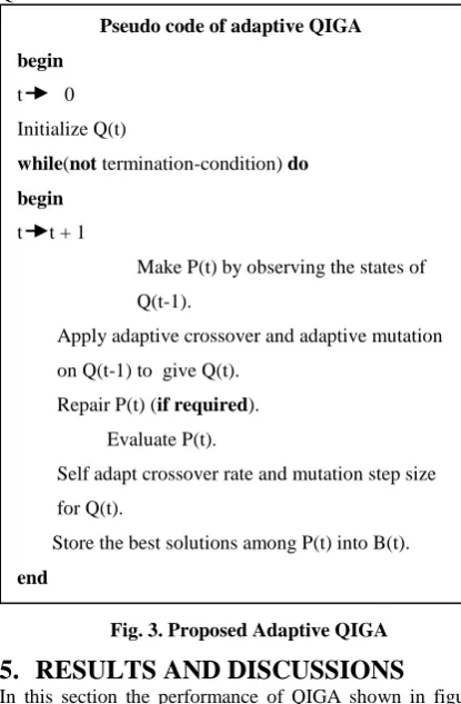
With the previously described components of GA, representation of individuals in QIGA and adaptation on QIGA, the proposed adaptive QIGA is presented in figure 3. Table 1 describes variants of QIGAs and adaptive QIGAs for which experiments are conducted in this paper. Table 2 shows parameter used for the conventional QIGA and adaptive QIGA.

Fig. 3. Proposed Adaptive QIGA

5.

RESULTS AND DISCUSSIONS

In this section the performance of QIGA shown in figure 4 and adaptive QIGA techniques are compared for different combinatorial optimization problems, namely, Knapsack, Maxcut and Onemax problems. Table 1 presents the different types of QIGA used in this work.

While executing the algorithms the best fitness/ profit achieved is plotted against the iteration number. To compare the convergence of the described algorithms in Table 1, each algorithm is executed 30 times. Then best graph among these 30 runs is taken out for each and compared with all other algorithms.

To study the time efficiency of these algorithms, they are executed with different population sizes and the time elapsed for each algorithm with different population sizes is recorded. These time graphs are then compared with each other.

Pseudo code of adaptive QIGA

begin

t 0 Initialize Q(t)

while(not termination-condition) do

begin

t t + 1

Make P(t) by observing the states of Q(t-1).

Apply adaptive crossover and adaptive mutation on Q(t-1) to give Q(t).

Repair P(t) (if required). Evaluate P(t).

Self adapt crossover rate and mutation step size for Q(t).

Store the best solutions among P(t) into B(t). end

5.1

Knapsack Problem

First benchmark problem taken in this work is Knapsack problem. In knapsack problem, there are „n‟ items, each of which is associated with weight and profit pair. Then select or reject each item in order to maximize total profit while total weight should not exceed by a certain bound.

Mathematical formulation of this problem is shown below [20-21].

Max 𝐧𝐢=𝟏𝐩𝐢𝐱𝐢

Such that 𝐧𝐢=𝟏𝐰𝐢𝐱𝐢≤ 𝐜 xiЄ{0,1}

pi>=0 and wi>=0 i=1,2...,n

Where pi is the profit on ith item and wi is the weight of ith item.

(a) Number of items are 24

(b) Number of Items are 100

(c) Number of Items are 250

(d) Number of Items are 500

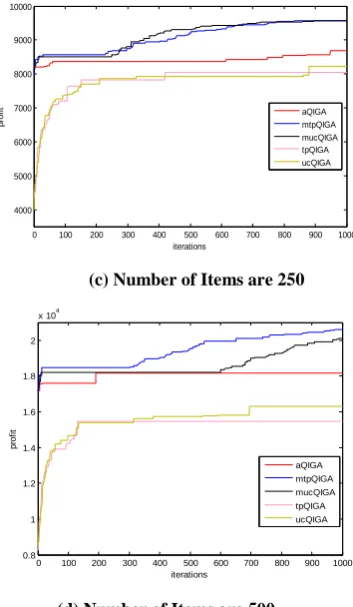
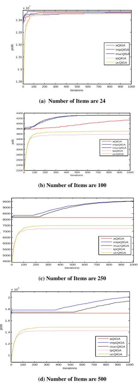
Fig. 5. Comparisons of Various QIGAs and Adaptive QIGAs on Best Profit vs. Number of Iterations Graphs for

Knapsack Problem with Parameter Setting shown in Table 2.

Experiments were conducted for the following problem instances: 24, 100, 250 and 500. Figure 5 and 6 shows the performance of the algorithms on knapsack problem. Figure 5 plots best profit vs. number of iterations and figure 6 plots the average profit vs. number of iterations for variants of QIGA and adaptive QIGA. In both figure 5 and figure 6, part (a) is for item size 24, (b) for 100, (c) for 250 and (d) for 500. In general, figure 5 shows that the adaptive QIGAs with all adaptation gives better results than the conventional QIGAs in terms of convergence to optimal values. According to figure 5

(a) all the algorithms converges to the optimum value for a small sized problem, while figure 5 (b), (c), (d) show that adaptive QIGA converges to higher values than the conventional QIGAs. However, even though aQIGA gives good results than conventional QIGA converges prematurely to some local optima and is not able to escape from that optima. But, this is not the case with mtpQIGA and

0 100 200 300 400 500 600 700 800 900 1000 1.22

1.24 1.26 1.28 1.3 1.32 1.34 1.36x 10

7

iterations

p

ro

fi

t

aQIGA mtpQIGA mucQIGA tpQIGA ucQIGA

0 100 200 300 400 500 600 700 800 900 1000 2000

2500 3000 3500 4000 4500

iterations

p

ro

fi

t

aQIGA mtpQIGA mucQIGA tpQIGA ucQIGA

0 100 200 300 400 500 600 700 800 900 1000 4000

5000 6000 7000 8000 9000 10000

iterations

p

ro

fi

t _aQIGA

mtpQIGA mucQIGA tpQIGA ucQIGA

0 100 200 300 400 500 600 700 800 900 1000 0.8

1 1.2 1.4 1.6 1.8 2

x 104

iterations

p

ro

fi

t

aQIGA mtpQIGA mucQIGA tpQIGA ucQIGA

Table 1

Variants of QIGA and Adaptive QIGA

QIGA

Description

aQIGA All adaptations on QIGA described in previous section

mtpQIGA Mutation step adaptation on QIGA with two point crossover

mucQIGA Mutation step adaptation on QIGA with uniform crossover

tpQIGA QIGA with two point crossover ucQIGA QIGA with uniform crossover

mtpQIGA Mutation step adaptation on QIGA with two point crossover

Table 2

Parameters for QIGA and Adaptive QIGA

Parameter Value

Maximum iterations 1000

Population size 50

Initial crossover rate 0.5

Mutation rate(conventional QIGA) 0.1

1st crossover point n/3

2nd crossover point 2*n/3

values. These figures also show that uniform crossover works well with conventional QIGA and using two point crossover with mutation step adaptation on QIGA gives the best results for knapsack problem among all kinds of QIGAs.

(a) Number of Items are 24

(b) Number of Items are 100

(c) Number of Items are 250

(d) Number of Items are 500

Fig. 6. Comparisons of Various QIGAs and Adaptive QIGAs on Average Profit vs. Number of Iterations

Graphs for Knapsack Problem with Parameter Setting shown in Table 2.

5.2

Maxcut Problem

Second benchmark problem used here is Maxcut problem. Maxcut problem is graph based problem, in which there is a weighted graph and find two disjoint subsets of that graph (or partition of the graph) in such a way that the sum of the weights wij on the edges going from one subset to another is maximized. In this work, the representation of the solution for this problem is taken as the binary string (x1, x2,…,xn) where each digit corresponds to a vertex. If a digit is 1 then hat vertex is said to be included in subset 1, otherwise it is said to be included in subset 2 [22]. Mathematical formulation of this problem is shown below.

Max 𝐢=𝟏𝐧−𝟏 𝐧𝐣=𝐢+𝟏𝐰𝐢𝐣. [𝐱𝐢(𝟏 −𝐱𝐣) + 𝐱𝐣(𝟏 − 𝐱𝐢)] Such that xi, xjЄ{0,1}

Experiments were conducted for the following problem instances: nodes 80 and edges 3128, nodes 125 edges 375, nodes 216 edges 648. Figure 7 and 8 shows the performance of the algorithms on Maxcut problem. Figure 7 plots best fitness vs. number of iterations and figure 8 plots the average fitnesst vs. number of iterations for variants of QIGA and adaptive QIGA shown in Table 1 on Maxcut problem. In both figure 7 and figure 8, part (a) is for nodes 80 and edges 3128, (b) for nodes 125 edges 375, (c) for nodes 216 edges 648. In general, figure 7 shows that the adaptive QIGAs with all adaptation gives better results than the conventional QIGAs in terms of convergence to optimal values. According to figure 7(a) except mtpQIGA and mucQIGA all the algorithms converges to the same local optima for a small sized problem, while figure 7 (b), (c) show that adaptive QIGA converges to higher values than the conventional QIGAs. However, even though aQIGA gives good results than conventional QIGA converges prematurely to some local optima and is not able to escape from that optima. But, this is not the case with mtpQIGA and mucQIGA. They converge monotonically to the optimum values. These figures also show that uniform crossover works well for conventional QIGA as well as QIGA with mutation step adaptation for problem size 80 and 100 but for problem size 216, two point crossover gives good results with conventional QIGA as well as QIGA with mutation step adaptation.

(a) Number of Nodes are 80 with 3128 Edges

0 100 200 300 400 500 600 700 800 900 1000

1.29 1.3 1.31 1.32 1.33 1.34

x 107

iterations

p

ro

fit aQIGA

mtpQIGA mucQIGA tpQIGA ucQIGA

0 100 200 300 400 500 600 700 800 900 1000

2200 2400 2600 2800 3000 3200 3400 3600 3800 4000 4200 4400

iterations

pr

of

it

aQIGA mtpQIGA mucQIGA tpQIGA ucQIGA

0 100 200 300 400 500 600 700 800 900 1000

4500 5000 5500 6000 6500 7000 7500 8000 8500 9000 9500

iterations

pr

of

it

aQIGA mtpQIGA

mucQIGA tpQIGA

ucQIGA

0 100 200 300 400 500 600 700 800 900 1000

1 1.2 1.4 1.6 1.8 2

x 104

iterations

pr

of

it

aQIGA mtpQIGA mucQIGA tpQIGA ucQIGA

0 100 200 300 400 500 600 700 800 900 1000

40 60 80 100 120 140 160 180 200 220 240

iterations

fi

tn

e

s

s

(b) Number of Nodes are 125 with 375 Edges

(c) Number of Nodes are 216 with 648 Edges.

Fig. 7. Comparisons of Various QIGAs and Adaptive QIGAs on Best Profit vs. Number of Iterations Graphs for

Maxcut Problem with Parameter Setting shown in Table 2.

(a) Number of Nodes are 80 with 3128 Edges

(c) Number of Nodes are 216 with 648 Edges.

Fig. 8. Comparisons of Various QIGAs and Adaptive QIGAs as on Average Profit vs. Number of Iterations Graphs for Maxcut Problem with Parameter Setting

Shown in Table 2.

5.3

Onemax Problem

The third benchmark problem used is Onemax problem. The Onemax problem consists of maximizing the number of ones of a bit string. The optimum value is 1*n, where n is the length of the bit string. Mathematical formulation of this problem is shown below.

Max 𝒏𝒊=𝟏𝒙𝒊 Such that xi Є{0,1}

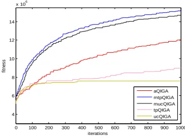
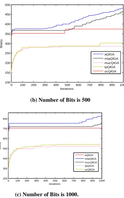
Experiments were conducted for the following problem instances: bit string length 50, bit string length 500 and bit string length 1000. Figure 9 and 10 show the performance of the algorithms on Onemax problem. Figure 9 plots best fitness vs. number of iterations and figure 10 plots the average fitnesst vs. number of iterations for variants of QIGA and adaptive QIGA shown in Table 1 on Onemax problem. In both figure 9 and figure 10, part (a) is for bit string length 50, (b) for bit string length 500, (c) for bit string length 1000. In general, figure 9, 10 show that the adaptive QIGAs with all adaptation gives better results than the conventional QIGAs in terms of convergence to optimal values. According to figure 9 (a), (b) and (c) show that adaptive QIGA converges to higher values than the conventional QIGAs. However, even though aQIGA gives good results than conventional QIGA converges prematurely to some local optima and is not able to escape from that optima. But, this is not the case with mtpQIGA and mucQIGA. They converge monotonically to the optimum values. These figures also show that uniform crossover works well with conventional QIGA and using two point crossover with mutation step adaptation on QIGA gives the best results for onemax problem among all kinds of QIGAs.

(a) Number of Bits is 50

0 100 200 300 400 500 600 700 800 900 1000

2 3 4 5 6 7 8 9 10 11x 10

6

iterations

fit

ne

ss

aQIGA mtpQIGA mucQIGA tpQIGA ucQIGA

0 100 200 300 400 500 600 700 800 900 1000

0.4 0.6 0.8 1 1.2 1.4 1.6

x 107

iterations

fi

tn

e

s

s

aQIGA mtpQIGA mucQIGA tpQIGA ucQIGA

0 100 200 300 400 500 600 700 800 900 1000

60 80 100 120 140 160 180 200

iterations

fit

ne

ss

aQIGA mtpQIGA mucQIGA tpQIGA ucQIGA

0 100 200 300 400 500 600 700 800 900 1000 2

3 4 5 6 7 8 9 10x 10

6

iterations

fi

tn

e

s

s

aQIGA mtpQIGA mucQIGA tpQIGA ucQIGA

0 100 200 300 400 500 600 700 800 900 1000 4

6 8 10 12 14

x 106

iterations

fi

tn

e

s

s

aQIGA mtpQIGA mucQIGA tpQIGA ucQIGA

0 100 200 300 400 500 600 700 800 900 1000

20 25 30 35 40 45 50

iterations

fit

ne

ss

(b) Number of Bits is 500

(c) Number of Bits is 1000.

Fig. 9. Comparisons of Various QIAGs and Adaptive QIGAs on Best Profit vs. Number of Iterations Graphs for Onemax Problem with

Parameter Setting shown in Table 2.

5.4

Time Graphs

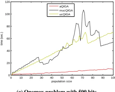
Graphs in figure 11 show the comparison of time to maximum number of generations taken by various QIGAs with adaptive QIGAs for Knapsack, Maxcut and Onemax problems. The maximum number of generations was fixed to 1000. The algorithms were compared for different population sizes. For Knapsack problem, the graph in figure 11 (a) with number of items 250 shows that conventional QIGA with two point crossover takes least time, while adaptive QIGA with two point crossover and mutation step adaptation takes maximum time. Adaptive QIGA lies in between these two algorithms. For Maxcut problem, the graph in figure 11 (b) with number nodes 80 and number of edges 3128 shows that adaptive QIGA takes least time, while QIGA with uniform crossover and mutation step adaptation takes less time than conventional QIGA with population size 11-50 and 85-100.

For Onemax problem, the graph in figure 11 (c) with bit string length 500 shows that adaptive QIGA takes least time, while QIGA with uniform crossover and mutation step adaptation takes less time than conventional QIGA with population size 25-55 and 88-100.

(a) Number of Bits is 50

(b) Number of Bits is 500

(c) Number of Bits is 1000

Fig. 10. Comparisons of Various QIAGs and Adaptive QIGAs on Average Profit vs. Number of Iterations Graphs for Onemax Problem with Parameter Setting

shown in Table 2.

(a) Knapsack Problem with Number of Items = 250

0 100 200 300 400 500 600 700 800 900 1000

100 150 200 250 300 350 400 450 500

iterations

fi

tn

e

s

s

aQIGA mtpQIGA mucQIGA tpQIGA ucQIGA

0 100 200 300 400 500 600 700 800 900 1000 200

300 400 500 600 700 800

iterations

fi

tn

e

s

s

aQIGA mtpQIGA mucQIGA tpQIGA ucQIGA

0 100 200 300 400 500 600 700 800 900 1000 20

25 30 35 40 45 50

iterations

fi

tn

e

s

s

aQIGA mtpQIGA mucQIGA tpQIGA ucQIGA

0 100 200 300 400 500 600 700 800 900 1000 150

200 250 300 350 400 450

iterations

fi

tn

e

s

s

aQIGA mtpQIGA mucQIGA tpQIGA ucQIGA

0 100 200 300 400 500 600 700 800 900 1000

200 300 400 500 600 700 800

iterations

fit

ne

ss

aQIGA mtpQIGA

mucQIGA tpQIGA ucQIGA

0 10 20 30 40 50 60 70 80 90 100

0 50 100 150 200 250 300 350

population size

tim

e

(s

ec

.)

aQIGA

mtpQIGA

(b) Maxcut Problem with 80 Nodes and 3128 Edges

(c) Onemax problem with 500 bits.

Fig. 11. Time vs. Population Size Graphs with Various QIGAs and Adaptive QIGAs.

5.5

Convergence and Success Rate

Additional experiments were carried out for the algorithms in Table 1 shown in appendix 1 for the benchmark problems. The results of these experiments are presented in Table 3. The problem instances used were different from the ones described in the previous sections. The parameter setting for the QIGAs is same as described in Table 2. Following inferences can be drawn from the results obtained:

1) Number of iterations taken by adaptive QIGAs to reach the optimal solution is less than that for the conventional QIGAs which shows that the adaptive QIGAs converge to the optimal solutions faster than the conventional QIGA. 2) The difference of the optimal solution obtained with

adaptive QIGAs and known optimal solution is less than that with the conventional QIGAs.

3) Also, the success rate of getting an optimum solution (number of occurrences of the optimal solution in the population before termination) is higher for adaptive QIGAs.

4) Mean fitness of the solutions obtained is also calculated which shows that on an average adaptive QIGA gives better results than conventional QIGAs in each iteration. The experiments were conducted on the variants of QIGAs and adaptive QIGAs with various small as well as large problem instances and it was found that adaptive QIGAs works well for both types of problem instances.

6.

CONCLUSION

Effectiveness and efficiency of an evolutionary algorithm depends on many factors, for example, representation of the solutions, operators, variation in operators, parameter settings etc. Among these factors the adequate parameter setting affects the performance of the algorithm very much. Therefore, the adaptive control on strategy variables in Genetic algorithm and hence in QIGA plays an essential role for successful search process.

In this work, adaptation of various parameters in QIGA is presented that self adapts crossover type, crossover rate and mutation step size. The experiments on the benchmark problems (namely 0/1 Knapsack problem, Maxcut problem and Onemax problem) have been attempted with variants of QIGA and adaptive QIGA. The experiments shows that with the choice of proper adaptive control parameters in QIGAs increase the efficiency of the algorithm and decrease the tasks done manually that leads to inaccuracy and very much time consumption. It is also found that adaptive QIGAs converge faster than the conventional QIGA and give better results. The work can be extended in the following directions:

i.Implement parallel adaptive QIGA to make it time efficient.

ii. Apply adaptation on other parameters of QIGA e.g. population size, mutation rate, selection procedure etc., so that it can converge rapidly to the optimal value.

7.

REFERENCES

[1] Sean Luke, Essentials of Metaheuristics: A Set of Undergraduate Lecture Notes, Department of Computer Science George Mason University, 2012.

[2] Ko Hisn Liang, Xin Yao and Charls S. Newton, “Adapting Self-Adaptive Parameters in Evolutionary Algorithms”, Applied Intelligence, 15, 1771-180, Kulwer Academic Publisher, 2001.

[3] Imtiaz Korejo, Shengxiang Yang and Chaanghe Li, “A Comparative Study of Adaptive Mutation Operators for Genetic Algorithm”, Metaheuristic International Conference, Hymberg, Germany July 13-16, 2009. [4] B. Rylander, T. Soule, J. Foster, J. Alves-Foss, “

Quantum Genetic Algorithms”. In Proc. GECCO, pp. 373- 377, 2000.

[5] Tzung-Pei Hong , Hong-Shung Wang , Wen-Yang Lin , Wen-Yuan Lee, “Evolution of Appropriate

Crossover and Mutation Operators in a Genetic Process”, Applied Intelligence, v.16 n.1, p.7-17, January-February

2002.

[6] Huaixiao Wang, Jianyong Liu, Jun Zhi and Chengqun Fu, “The Improvement of Quantum Genetic Algorithm and Its Application on Function Optimization”, Mathematical Problems in Engineering, Volume 2013, 2013.

[7] S. Meyer-Nieberg and H.G. Beyer, “Self- Adaptation in Evolutionary Algorithms”, Studies in Computational Intelligence (SCI) 54, 47–75, Springer- Verlag Berlin

Heidelberg 2007.

[8] Oliver Kramer, “Evolutionary Self- Adaptation: A Survey of Operators and Strategy Parameters”, Evolutionary Intelligence, pp. 51-65, 2010.

0 10 20 30 40 50 60 70 80 90 100

0 10 20 30 40 50 60 70 80 90

population size

ti

m

e

(

s

e

c

.)

aQIGA mucQIGA ucQIGA

0 10 20 30 40 50 60 70 80 90 100

0 20 40 60 80 100 120

population size

ti

m

e

(

s

e

c

.)

[9] Renato Tin´os and Shengxiang Yang, “Self- Adaptation of Mutation Distribution in Evolutionary Algorithms”, IEEE Congress on Evolutionary Computation, 2007. [10]Bartlomeij Gloger, Lecture notes on Self Adaptive

Evolutionary Algorithms,University of Paderborn, 2004.

[11]Wen-Yanglin, Wen-Yuanlee and Tzung-Peihong, “Adapting Crossover and Mutation Rates in Genetic Algorithms”, Journal of Information Science and Engineering 19, pp. 889-903 ,2003.

[12]Kuk-Hyun Han and Jong-Hwan Kim, “Quantum-inspired Evolutionary Algorithm for a Class of Combinatorial Optimization”, IEEE transaction on Evolutionary Computation, Vol. 6, No. 6, December 2002.

[13]D. Ashlock, Evolutionary Computation for Modeling and Optimization, Springer, ISBN 0-387-22196-4, 2006. [14]U.V. Vazirani, lecture notes on Qubits, Quantum

Mechanics, and Computers for Chem/CS/Phys191, University of California, Berkeley, 2012. www.cs.berkeley.edu/~vazirani/.

[15] Mark Oskin, Quantum Computing- Lecture Notes, Department of Computer Science and Engineering, University of Washington, Washington. homes.cs.washington.edu/~oskin/.

[16]Kuk-Hyun Han and Jong-Hwan Kim, “Analysis of Quantum Inspired Evolutionary Algorithm”,

Proceedings of International Conference on Artificial Intelligence, 2001.

[17]James E. Smith, “Self- Adaptation in Evolutionary Algorithms for Combinatorial Optimization”, Adaptive and Multilevel Metaheuristics Studies in Computational Intelligence, Volume 136, 2008, pp 31-57, 2008. [18]S. Uyar, G. Eryigit, S. Sariel, “An Adaptive Mutation

Scheme in Genetic Algorithms for Fastening the Convergence to the Optimum”, Proceedings of the

3rd Asia Pacific International Symposium on Information Technology, pp. 461–465, 2004. [19]W. M. Spears,., “Adapting Crossover in a Genetic

Algorithm”, Naval Research Laboratory AI Center Report AIC-92-025, Washington, DC 20375, USA, 1992.

[20]Hristakeva, Maya and Dipti Shrestha. “Solving the 0/1 Knapsack Problem with Genetic Algorithms.” MICS 2004 Proceedings, 2004.

[21]Megha Gupta, “A Fast and Efficient Genetic Algorithm to Solve 0-1 Knapsack Problem”, International Journal of Digital Application & Contemporary research, Volume 1, Issue 6, January 2013.

[22]Enrique Alba and Bernabe Dorronsoro, Cellular Genetic Algorithms, © Springer Science+ Business Media, LLC, pp. 213-219, 2008.

8.

AUTHOR BIOGRAPHY