Image compression using noncausal prediction

Rochester Institute of Technology

RIT Scholar Works

Theses

Thesis/Dissertation Collections

4-1-1998

Image compression using noncausal prediction

J. F. Marchand

Follow this and additional works at:

http://scholarworks.rit.edu/theses

This Dissertation is brought to you for free and open access by the Thesis/Dissertation Collections at RIT Scholar Works. It has been accepted for

inclusion in Theses by an authorized administrator of RIT Scholar Works. For more information, please contact

[email protected]

.

Recommended Citation

Image Compression using Noncausal Prediction

By

J.

F. Philippe Marchand

Rochester Institute of Technology

(1998)

A dissertation submitted in partial fulfillment of the

requirements for the degree of Ph.D.

in the Chester

F.

Carlson Center for Imaging Science

of the College of Science

Rochester Institute of Technology

April 1998

Signature of Author,

~

---,

Accepted by

Henry E. Rhody

Coordinator, Ph.D. program

;tf~

2 2 /

197('

CHESTER F. CARLSON

CENTER FOR IMAGING SCIENCE

COLLEGE OF SCIENCE

ROCHESTER INSTITUTE OF TECHNOLOGY

ROCHESTER, NEW YORK

CERTIFICATE OF APPROVAL

Ph.D DEGREE DISSERTATION

The Ph.D. Degree Dissertation of J.F. Philippe Marchand

has been examined and approved by the

dissertation committee as satisfactory for the

dissertation requirement for the

Ph.D degree in Imaging Science

Dr. Harvey Rhody, Thesis Advisor

Dr.Steven McLaughlin

Dr. Roger Easton

Dr. Raghuveer Rao

Dr. Peter Crean

DISSERTATION RELEASE PERMISSION

ROCHESTER INSTITUTE OF TECHNOLOGY

COLLEGE OF SCIENCE

CHESTER F. CARLSON

CENTER FOR IMAGING SCIENCE

Title of Dissertation:

Image Compression using Noncausal prediction

I, J.F. Philippe Marchand, prefer to be contacted each time a request for reproduction is

made. I can be reached at the following address:

J.F. Philippe Marchand

PO Box 473

Webster, NY 14580, USA

Abstract

Image

compression

commonly

is

achieved

using

prediction

of

the

value of

pixels

from

surrounding

pixels.

Normally

the

choice

of

pixels

used

in the

prediction

is

restricted

to

previously

scanned pixels.

A

better

prediction

can

be

achieved

if

pixels on

all

sides of

the

pixel

to

be

predicted are

used.

A

prediction and

decoding

method

is

proposed

that

is

independent

of

scanning

order of

the image.

The

decoding

process makes

use of an

iterative

decoder. A

sequence

of

images is

generated

that

converges

to

a

final image

that

is identical to the

original

image. The

theory

underlying

noncausal prediction and

iterative

decoding

is developed. Convergence

properties of

the

decoding

algorithm

are

studied and conditions

for

convergence are

presented.

Distortions to the

prediction residual after

encoding

can

be

caused

by

storage

requirements,

such

as

quantization

and

compression and also

by

errors

in

transmission.

Effects

of

distortions

of

the

residual on

the

final decoded image

are

investigated

by introducing

several

types

of

distortion

of

the

residual,

including (1)

alteration of

randomly

selected

bits in the

residual,

(2)

addition of

a

sinusoidal signal

to

the

residual,

(3)

quantization of

the

residual

and

(4)

compression of

the

residual

using

lossy

Haar

wavelet coding.

The

resulting

distortion

in

the

decoded

images

was

generally

less for

noncausal prediction

than

for

causal

prediction,

both in terms

of

PSNR

and

visual quality.

Most

noticeably,

the

streaks

found

in the decoded Image

after

ACKNOWLEDGEMENTS

I

wish

to

acknowledge

Dr.

Harvey Rhody

for

his

help

with

the

research

and

the

writing

of

this

dissertation.

I

wish

to

acknowledge

Xerox

Corporation for

supporting my

studies at

the

Chester F.

DEDICATION

Table

of contents

Chapter

1

Introduction

1

1

.1

Overview

of

Literature

6

Chapter 2

Prediction-Based

Coding

10

2.1

Conventional linear

predictive

coding

1 2

2.2.

Image

Quality

Measures

14

2.3.

Entropy-based

performance measure

16

Chapter 3

Decoding

with

Causal Predictors

17

Chapter 4

Decoding

Methods

19

4.1 Iterative

Decoding

Method

20

4.2

Constrained Iterative

Reconstruction Algorithm

27

4.3 Direct

Decoding

32

Chapter 5

Decoding

using

quantized

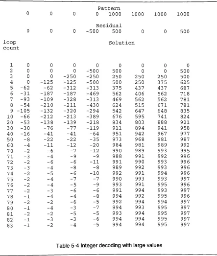
representation of residual

35

5.1

Problems

with

integer

representationof residual

35

5.2 Error

analysis

40

5.3 One-dimensional

error simulation

42

5.4

Worst

Case

error

45

5.5 Error for Random

truncation

45

Chapter

6

Results

52

6.1

Test

plan

54

6.2 Effect

of

adding

random

bit-flips to

the

residual

56

6.4 Linear

Quantizer

64

6.5 Nonlinear

Quantizer:

Lloyd-Max

optimization

68

6.6

Optimizing

the

noncausal prediction

coefficient a

70

6.7

Mathematica Simulation

73

6.8 Effect

of

adding

sinewaves

to

the

residual

77

6.9 Effect

of

compressing

the

residual

with

the

Haar

wavelet

transform

81

6.10 Description

of program

"Image"

85

Chapter 7

Summary

88

7.1

Suggestions for future

work

90

Table

of

Figures

and

Tables

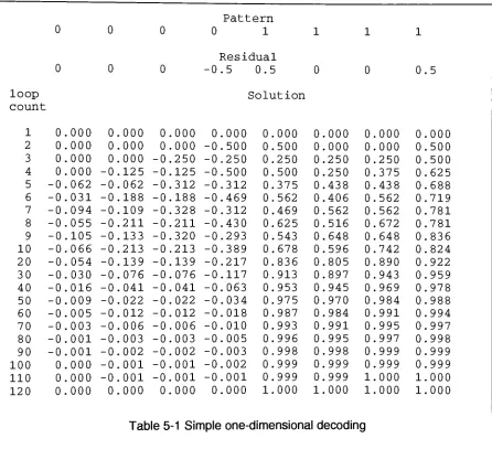
Table

5-1

Simple

one-dimensional

decoding

36

Table

5-2

Decoding

with

integer

valued

pixels,

using

truncation

38

Table

5-3

Decoding

with

integer

valued

pixels,

using

truncation:

38

Table

5-4

Integer

decoding

with

large

values

39

Table

5-5

Error

sums and

PSNR for

worst case and random

48

Table

6-1 RMS Distortion

and

PSNR

of

the

decoded image

78

Figure 1-1

The

neighborhood

of pixel

X

2

Figure

2-1 Basic

prediction

block diagram

10

Figure 2-2 Compression

added

to

prediction

1

1

Figure 2-3 Channel

errors added

to

prediction

1 1

Figure 2-4 Pixel

neighborhood

12

Figure 3-1 Pixel

neighborhood

17

Figure

4-1 Iteration Model

20

Figure

4-2 Encoder

21

Figure

4-3

Iterative decoder

21

Figure 4-4 The

noncausal predictor

in

matrix

form

26

Figure 4-5 Contraction

mapping

29

Figure 4-6 Convergence

of

iteration

process

31

Figure

5-1

Two-dimensional

image

42

Figure

5-2

One-dimensional

image

42

Figure 5-3 Peak

value of

impulse

response

44

Figure

5-4

Magnitude

of

impulse

response

44

Figure 5-5

RMS

error as

function

of a

46

Figure 5-6 First-order

entropy Hi

of

residual

vs.

a,

for image

"Lena"

47

Figure 5-7 The 1

-D

impulse

response

of residual

impulse

at n=0

49

Figure 5-8

Same

as

Figure

5-7,

but

with

entry

for

a=0.50

removed

50

Figure 5-9 1D

error

image from

rounded residual

for 0.49

>a>

₀

51

Figure 6-1 The

test

plan

54

Figure 6-2

Adding

random

bit-flips to

residual

image

56

Figure

6-3

Using

a median

filter to

reduce

the

effect

of

the

random

bit

flips

58

Figure 6-4 Decoded image. 132

random

bit flips. Predictor is

noncausal

59

Figure

6-5 Decoded image. 132

random

bit flips. Predictor is

causal

59

Figure 6-6 Error in decoded image. 132

random

bit flips. Predictor is

noncausal

59

Figure 6-7 Error in decoded image. 132

random

bit flips. Predictor

is

causal

59

Figure 6-8 Decoded image. 132

random

bit flips. Predictor is

noncausal +

5-pixel

median

filter

applied

to the

residual

60

Figure

6-9

Decoded image. 132

random

bit flips. Predictor is

causal +

5-pixel

median

filter

applied

to the

residual

60

Figure 6-10 Error in decoded image. 132

random

bit flips. Predictor

is

noncausal

+

Figure 6-1 1

Error

in decoded

image.

132

random

bit

flips.

Predictor is

causal +

5-pixel

median

filter

applied

to the

residual

60

Figure

6-12

Signal-to-noise

ratio of

decoded

image

with

bit

errors

in the

residual

image.

61

Figure 6-13

Quantization

of

the

residual

63

Figure

6-14

The

causal and

the

noncausal predictors

64

Figure 6-15 Decoded image

with

quantized residual, quantization step=20.

Predictor

is

noncausal

66

Figure 6-16 Decoded image

with

quantized

residual, quantization step=20.

Predictor is

causal

66

Figure 6-17 Error in decoded image

with

quantized

residual, quantization step=20.

Predictor is

noncausal

66

Figure

6-18

Error in decoded image

with

quantized

residual, quantization

step=20.

Predictor

is

causal

66

Figure 6-19

Quality

of

decoded image for

causal

and

noncausal

predictors

67

Figure 6-20.

Quality

of

decoded

image for

causal

and

noncausal

predictors

using

uniform quantizationand

Lloyd-Max

optimized quantization

69

Figure 6-21 The PSNR

as a

function

of

entropy for

several values of a

71

Figure 6-22 The PSNR

as

a

function

ofa

for

two

values of

the

resulting

first-order

entropy

72

Figure 6-23 Impulse

response

of

error

in

residual

for

noncausal prediction

74

Figure 6-25

Impulse

response

for

causal and

noncausal

prediction

for

different

sizes

of

the

image

76

Figure 6-26

Adding

a sinusoidal signal

to

residual

image

77

Figure

6-27

Decoded

image

with

noncausal

predictor;

f=2,

amplitudes

0

79

Figure 6-28

Decoded image

with

noncausal

predictor;

f=64,

amplitudes

0

79

Figure

6-29 Error in

decoded image

with

noncausal

predictor;

f=2,

amplitude=10

79

Figure

6-30 Error in decoded

image

with noncausal

predictor;

f=64,

amplitude=10

79

Figure

6-31 Decoded image

with

causal

predictor;

f=2,

amplitude=10

80

Figure

6-32 Decoded image

withcausal

predictor;

f=64,

amplitudes

0

80

Figure

6-33 Error in decoded image

with causal

predictor;

f=64,

amplitudes

0

80

Figure 6-34 Error in decoded image

withcausal

predictor;

f=2,

amplitude^

0

80

Figure

6-35

Compressing

the

residual

with

the Haar

wavelet

transform

82

Figure

6-36 PSNR

vs.

file-size

for

several values of

the

quantization

step-size

for the

Haar

wavelet coefficients

83

Figure 6-37 Decoded image

with noncausal predictor

and

residual

that

was

compressed

with

the Haar

wavelet.

Quantization

step=25

84

Figure 6-38 Decoded

image

with causal predictor

and residual

that

was

compressed

with

the Haar

wavelet.

Quantization

step=25

84

Figure 6-39 Error in decoded image

above.

PSNR=27dB

84

Chapter

1

Introduction

Images

are

commonly

stored and

transmitted

in digital form

by

assigning

a value

to

each of

the

picture elements

(pixels)

of

the

image.

These

pixel values

are

then

stored

in

computer

files

or

transmitted

over communication channels.

Because

there

are

many

pixels

in

an

image the

files

become large

and a

large

amount

of

bandwidth

is

needed

to

transmit the images. Image

compression

attempts

to

reduce

the

number of

bytes

needed

to

represent

the

image

and

thus

reduce

the

requirements

for

storage

and

bandwidth.

Linear

prediction

may be

used as an element of

image

or signal compression.

Predictive

techniques that

were

developed for

random signals

and

time

series

have

been

adapted

for

use with

images. The

essential

idea is to

use

a

model of

the

process

to

predict

the

next value

in

a

data

sequence

based

on current

and past

values.

The

difference between

the

actual and predicted

value,

called

the residual,

contains

the

prediction error.

The

original

data

sequence can

be

reconstructed

from knowledge

of a

set of

initial

conditions and

the

residual sequence.

It

may

be

possible

to

encode

the

residual

for

storage or

transmission

with

fewer bits

than

would

be

required

for

direct

encoding

of

the

original

data,

particularly

by

simple

encoding

methods.

It is

a

means

that

may be

used

to

achieve a significant amount of compression

by

relatively

simple

processing.

Discrete

time

signals are sequences with a natural

past

and

future. To

apply

a process such as scanning.

Raster

scanning

is the

most

common

pattern,

but

others

are possible.

A

B

C

D

X

IL

E.

G_

H_

Figure 1-1 The

neighborhood

of pixel

X

If

an

image is

scanned

in

row order

from

top

to

bottom,

then

pixel

X in Figure

1-1 is

encountered

after

D but before E.

Preceding

values such as

A,

B,

C

and

D

can

be

used

to

predict

the

value of

X

that

will

be

seen

by

the scanner, but

E, F,

G

and

H

can

be

used

only

if

a

delay

buffer is

used.

Use

of

a

buffer

poses no

difficulty

for image

encoding, but it does

create a

problem

for

reconstruction.

In effect, the

reconstruction

algorithm needs

to

make use of values

that

have

not yet

been determined. In

causal

prediction pixel values

surrounding

the

pixel

to

be

predicted

are used

in the

prediction

process,

as shown

below:

Predicted

value of

X

:

P

=

CaA

+

CbB

+

CCC

+

CdD

(1-1)

Residual

R

=

X-P

=

X

-

(CaA

The

predictor model

is

defined

by

the

coefficient

values.

If

the

values are

fixed

they

may

be

chosen

to

minimize

the

prediction

error over

a sample

of representative

images.

If

they

are adjustable

they

can

be

changed

by

an adaptive process

to

reflect

changes

in

image

statistics.

In

any

case,

they

rely

on

the

idea that

the

near

future

can

be

predicted

by

the

present and

recent past.

Usually

the

change

in

value

from

one

pixel

to the

next

is

small.

Sudden

changes

in

the

value of

the

pixels occur when

the

image

has

edges

or other special

features.

In

noncausal prediction pixel values

surrounding

the

pixel

to be

predicted are

used

in the

prediction

process,

as

shown

below:

Predicted

value of

X

:

P

=

CaA

+

CbB

+

CCC

+

CdD

+

CeE

+

C,F

+

CgG

+

ChH

(1

_-3)

Residual

R

=

X-P

=

X

-

(CaA

+

CbB

+

CCC

+

CdD+

CeE

+

C,F

+

CgG

+

ChH)

(1

_-4)

The

noncausal predictor

has

the

causal predictor as a subset.

Therefore

a

noncausal predictormustgive results

that

are

statistically better

than those

available

to

the

causal predictor.

The

key

issue to be

addressed

is the

problem of

reconstructing

the

image from

the

residual produced

by

a

noncausal predictor.

The

purpose of

the decoder

is to

reconstruct

the

original

image

from

the

residual

image.

The

residual

is

again

scanned

from

left

to

right and

from

top

to bottom.

At

each pixel

location the

value of pixel

X is

Causal

prediction:

X=R

+

(CaA

+

CbB

+

CCC

+

CdD)

(1

-5)

Noncausal

prediction*

=

R

₊

(CaA

₊

CbB

₊

CCC

₊

CdD+ CeE

₊

C,F

₊

CgG

₊

ChH)

(1

-6)

In the

causal case

(1-5)

this

can

easily

be implemented because the decoder

has

reconstructed

the

values

of

pixels

A,B,C

and

D

by

the time

it

needs

to

use

them

for

calculating

the

value of

X.

After

a

single pass

through

the image

the

original

image has

been

reconstructed.

But

with noncausal

predictors a

problem

arises

because the decoder

also needs

to

know the

values of pixels

E,F,G

and

H. The

reconstructed values of

these

pixels are

not

available when

it is

trying

to

reconstruct

the

value

for

pixel

X.

Hence the

name

noncausal.

The

noncausal

dilemma

can

be

avoided

by

using

an

iterative decoder. In

the

iterative

decoding

process

the decoder

canreconstruct

the

original

image

by

making

an

initial

guess of

the image. Rather

than

using

known

values

for the

noncausal

pixels

E,F,G

and

H

the

algorithm uses an estimate of

those

values.

Using

this

estimate

the

decoder then

can

apply

the

prediction

process, together

with

the

known residue, to

generate

a

new

image

that

is

closer

to the

original.

This

new

image is then

used

to

supply

the

values

E,F,G

and

H for

a

better

reconstruction of

the

original

image. The

decoder

thus

creates a sequence of

images.

It

will

be

shown

that the

image

sequence

converges under appropriate conditions.

The limit

of

the

sequence

is

an

image that is

In direct reconstruction, the

iterative

approach

is

replaced

by

a

single-step

process.

In the

case

of

unconstrained

iterative

decoding,

the

process

can

be

replaced

by

linear

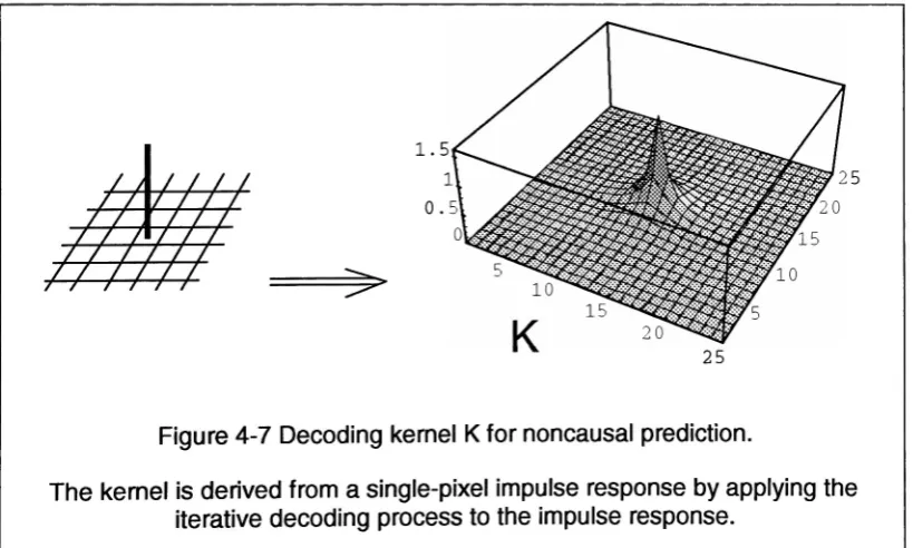
filtering. The

appropriate

linear

filter

is derived

by

creating

a

convolution of

the

residual

with

the

impulse

response

of

a single-unit

pixel

through

the iterative

decoding

process.

This

method

assumes

that

the

reconstruction

process

is

linear.

This

is

essentially

inverse

filtering,

where

the

reconstruction

filter

is

the

inverse

of

the

prediction

filter. The

process works

well

because

the

prediction

filter is known

exactly.

The inverse filter

is thus

obtained

by

performing

the

iterative

decoding

on

a single-unit

pixel.

The

residual

is

a complete

representation of

the full

image because the

original

can

be

restored

perfectly

by

the iterative decoding. We

are

therefore

interested in

the

question of

how

changes

in the

residual will affect

the

reconstruction.

Changes in

the

residual can

be

caused

by

lossy

compression or

transmission

errors.

The

effects of

distortion

of

the

residual

have been inspected for

several

kinds

of

distortion: integer

representation of

the residual,

quantization of

the residual,

and

lossy

compression of

the

residual

using

a

wavelet compression method.

Two

quantization

methods were used:

linear

quantization and nonlinearquantization

using

the

Lloyd-Max

optimization algorithm.

The

wavelet compression method uses

the

Haar

wavelet

transform

followed

by

linear

quantization and

Goulomb-Rice

coding.

Other distortions

of

the

residual

that

were

considered are:

intentional

corruptions

sine-waves

to the

residual.

In

all cases

the

effect

on

the

reconstruction

is

found

to be

a

"soft"

degradation. More

change

in the

residual produces more change

in the

reconstruction.

A

computer

program

called

"Image" was written

to

implement the

prediction

process and

the

reconstruction processes.

This

program

was used

for

evaluating

the

effects

of

distortion

of

the residual,

as

described

above.

The

program

Image

was

also

used

for

empirically

optimizing

the

prediction coefficients.

It

was

found

that there

is

an

optimum value

for the fourth

order noncausal prediction

coefficient

that

gives

the

best

tradeoff

between

compressed

file

size

of

the

residual

image

and

signal-to-noise

ratio

of

the

reconstructed

image.

A

simulation of

the

reconstruction

process

was also performed

using

the

program "Mathematica"

in

order

to look

at

the

effects

of noise

in the

residual on

the

reconstructed

image.

1

.1

Overview

of

Literature.

There

is

very

little

published

literature

that

deals

with

the

subject of noncausal

image

prediction

and

reconstruction.

Most

of

the

publishedwork

deals

with standard

scanning

sequences or special

scanning

schemes.

This

is different from the

approach

in this

dissertation,

where

the

images

are

treated

as whole

objects,

and

the

particular

scanning

sequence used

is

only incidental,

as

it is

needed

to

represent

the

image in

In

"Interpolative

DPCM",[7],

Sethia

and

Anderson

apply

noncausal prediction

in

an

Interpolative

DPCM

coder.

This

lossy

coder

is

applied

to

one

dimensional Laplacian

and

Gaussian

sources.

These

signals

are speech

like. The

authors report a

3 dB

improvement

in

signal-to-noise

Ratio

over

causal

DPCM. A

noncausal

interpolator

is

included in

a

closed-loop

coder.

An identical interpolator is

used

in the decoder. The

interpolator

looks

several samples

back

and one sample

forward. The

reconstruction

uses

a

direct interpolation

model rather

than

an

iterative

model.

Yuan,

Ingle,

and

Manolakis describe "An

adaptive

Image

Coding

Algorithm

based

on

Noncausal LPC

and

Vector

Quantization"

[12].

The

algorithm

is

applied

to

two-dimensional

images.

The

image

is

partitioned

into

blocks.

Noncausal

Linear

Predictive

Coding

analysis

is

performed

on

two-dimensional

image blocks

and

the

resulting

linear

predictors are

Vector Quantized.

The

residual

signals are computed

for

each

block

and coded

with an adaptive vector quantizer.

Spectrum

and

residual

energy

information from

the

LPC

codes

is

used

to

control

bit

allocation.

Experimental

results

show

that

good

coding

quality

can

be

achieved at

low

bit

rates.

This

method

implements

lossy

compression.

This

decoding

process

is

not

iterative.

M.

Khansari

has

a

PhD

thesis

and several publications on

the

subject

of

noncausal coding.

In

his PhD

thesis

[5]

"Block-Oriented Subband Decomposition

And

Linear

Interpolation

Source

Coding",

Khansari

refers

to

noncausal

prediction

as

Interpolation,

and

describes

methods

for

performing

perfect

reconstruction on

the

process.

The

rate

of

convergence

for

the

iterative

reconstruction process

is

also

determined

.

In

"Convolutional Interpolative

Coding

Algorithms"

[6], Khansari,

et al

describe

signal

coding

and

reconstruction

on

a one-dimensional

model of

a

two-dimensional

image source,

using

a second-order

noncausal predictor

(simple

interpolator).

The

algorithm uses

iterative

reconstruction

and

makes

use of

forward

and

backward

refinements,

where

the

iterative

process

is

applied

from

the

beginning

to the

end

and

from the

end

to the

beginning

of

the

sequence

of samples.

As

each

sample

is

updated,

it is

immediately

used

to

update of

the

next

sample.

This

paper also

discusses

quantization

effects

with

open-loop

and

closed-loop

coding.

The

method used

here

operates

within

the

sequence of

data

points.

It

does

not

treat the

image

as an object.

In "Noncausal

predictive

image

coding"

[1], Zhou,

Khansari

and

Leon-Garcia

expand

the

process

to two dimensional images. Perfect

reconstruction

is

achieved

with

an

iterative

reconstruction algorithm.

To

increase

the

rate

of

convergence,

the

"whirlpool"

algorithm

is introduced. The iteration is

performed

around

a number of

"fixed

points",

where

the

actual value of

the image is

transmitted to

the

receiver.

The

use of an entire

image

as

a "point"

in

the

reconstruction

process

gets

away

from

the

sequence of

data

withinan

image

viewpoint.

The

concept

of

the

"fixed

points"

analysis

in

Zhou,

et

al.,

could

be

embedded as a

constraint

in the

constrained

iterative

decoding

process proposed

in this

dissertation.

Note that the

"fixed

points"

referred

to

here

refer

to

pixels

in

an

image

that

have been transmitted

separately

to

facilitate

the

process,

which refer

to

whole

images

in

a

converging

sequence of

images.

The fixed

point

in the

iterative

reconstruction process

is the final image to

which

the

process

converges.

Balram

and

Moura

[8]

[21]

describe

a combination

of

interpolative

coding

and

vector

quantization.

The

residual

obtained

after

fourth-order

noncausal prediction

is

quantized

in

groups

of

4x4

pixels

using

64

code

vectors,

resulting

in

a

bitrate

of

0.375

bits

per pixel.

Schafer,

et

al.

[19]

describe

a general

framework for

performing

iterative

restoration on signals

that

were

distorted

with a

distortion

operator.

The distortion

operator,

or

its

approximation

matrix,

can

be

used

in

an

iteration

to

recover an

approximation

to the

original signal or

image.

Conditions

for

validity

and convergence

are

described. The

paper applies

the

process

to

several one-dimensional signals.

This

algorithm

is described in detail

and applied

to

iterative

decoding

in

chapter

4.

In

this

dissertation,

Schafer"s

constrained

iterative

restoration algorithm

is

used

as one

method

for

decoding

the

original

image from the

residual

obtained

through

noncausal prediction.

The

predictive

coding

process

replaces

the distortion to

be

eliminated.

The

method enables

the

use of constraints

that

can

be

used

to

enforce

known

boundary

conditions of

the

image,

like

the

fact

that the

value of

the

image

pixels

is

zero outside

its

boundaries

and

that

each pixel

is bounded in

value

between

a

minimum and

a

maximum value

(usually

0

and

255

respectively).

It

would

also enable

Chapter

2

Prediction-Based

Coding.

This

chapter presents

the

basic

concept

of predictive

coding,

which

is

a

method

to

reduce

the

amount

of

data

encoded

for

each

pixel so

that the

total

image

can

be

represented

with

fewer

bits.

Prediction-based coding

makes

use of

the

fact

that

for

most

images

there

is

a

relationship

between the

value of each pixel and

its

neighbors,

and

thus

knowing

the

values of

the

neighboring

pixels allows one

to

estimate or predict

the

value of

a

pixel.

It is

then

possible

to

specify

the

value of

that

pixel

merely

by

encoding

the difference between

the

actual value and

the

prediction.

Because

this

difference usually is

small,

fewer bits

are needed

to

represent

the

image.

The

residual

r

is

the

difference between the

original

image

x

and

the

image

formed

by

the

predicted

values,

as

illustrated in Figure 2-1

.

The

residual contains

the

same

information

as

the

original when

a

reconstruction

process exists

such

that

x'=x.

However,

the

residual will

have

a

lower first-order

entropy

and

its

use

may,

therefore,

lead to improved

overall performance when combined with common compression

algorithms such as

Huffman

encoders.

S V r I .

^

Prediction

TV

^

reconstruction

Figure 2-1 Basic

prediction

block diagram.

The

introduction

of compression

and

decompression

is illustrated in Figure 2-2.

The

compression and

decompression

can

be

either

lossless

or

lossy.

Lossless

input,

so

that r"=r,

from

which

x

can

be

recovered.

The

performance

measure of

interest

in that

case

is

simply

the

filesize

of rc

relative

to the

filesize

of x.

Lossy

compression

and

decompression

will

produce

an

output

rVr.

The

performance

measure

for

this

case

must account

for the

difference

x'-x

caused

by

the

difference

r"-r

and

compare

the

filesize

of rctox

Prediction

compression

de

compression

reconstruction

Figure 2-2

Compression

added

to

prediction

The difference between

causal

and

noncausal prediction

is in the

choice

of

the

weight

applied

to

surrounding

pixels

for

the

purpose

of prediction.

In

noncausal

coding,

any

pixel

in

the

whole

image

can

be

used,

whereas

in

causal

coding

the

choice of

pixels

is limited

to those that

have been

encoded

previously

in

the transmission

sequence.

The

noncausal approach

usually

allows

for better

prediction.

f

.

Prediction Transmissionchannel witherrors

decoding

Figure

2-3 Channel

errors added

to

prediction

The

introduction

of

a

lossy

transmission

channel

is introduced in Figure 2-3.

Errors in

the transmission

of

the

residual

from

the

predictor

to the

decoder

will

produce

an

output rVr

and

thus

x'*x.

The

performance measures

are

the

same as

in the

case

of

2.1

Conventional

linear

predictive

coding

Pi

x

p7

p5

Figure 2-4 Pixel

neighborhood

In

most

images,

there is

considerable

correlation

among

the

gray

values of

neighboring

pixels.

When

transmitting

the

value of pixel

X

(Figure

2-4),

it

is

possible

to

predict

its

value

from

neighboring

pixels and

transmit

only

the

difference between

the

prediction

and

the

actual value.

In

general

this

residual value can

be

encoded

with

fewer

bits

than

the

original

value,

resulting

in

image

compression.

A

common

way

to

predict

the

value of

pixel

X is

as a

weighted

average

of

the

surrounding

pixels.

For

images

with

few

sudden

changes

in

intensity (edges)

this

is

a

good assumption.

The

number of pixels considered

in

the

average

determines

the

"order" of

the prediction,

e.g.,

an eight order predictor uses all eight neighbors.

Better

prediction algorithms

produce

residuals with smaller variances and

lower

first-order

entropy

and

enable

higher

overall compression ratios with conventional compression algorithms.

Let

N(X)

be

a set

of points

in the image

used

to

predict

the

value of

X

for the

point

X

shown

in

Figure

2-4,

N(X)

=

(Pi(X),

P2(X),...Pn(X)}.

The

P,

are

usually

chosen

to

be

neighbors of

X,

but

may

be located

anywhere

in the image.

Let

V(X)

be the

value of

the

image

at a

point

X.

An

estimate of

V(X)

can

be

formed

from the

values of

the

pixels

in N(X). One

model

is

the

linear

sum:

V(X)=

2ciV(Pi)

PiN(X)

The

predictor model

is defined

by N(X)

and

the

coefficients

q.

The

residual

at

pixel

X is:

R(X)

=

V(X)-V(X).

(2-2)

The image

can

be

reconstructed

from

knowledge

of

R(X)

and

V(X)

.

The

estimate

V(X)

can

be

reconstructed

if

the

values

in

N(X)

have been

computed.

2.1.1

Scanning

sequence

Let

X(m)

be the

pixel

location

at

time

m.

The

scanning

process computes

the

residual

R(X(m))

in

an order

determined

by

the

sequence

X(m). The

particular

scanning

sequence

is

unimportant

as

long

as

each

pixel

in the

image is

visited

at

least

once.

All

scanning

sequences

contain

the

same

information,

and

may

be

considered

as

a

reordering

of some

base

sequence.

Reconstruction

of

the

value at pixel

X(m)

requires

that

V(X(m))

be

calculated

and added

to the

residual

V(X(m))

=

R(X(m))

+

V(X(m))

The

calculation can

be done

at

the

decoder

provided

that the

values

in

N(X(m))

are

known.

Let

D(m)

=

{

X(l),X(2),...X(m)

}

be

the

set

of

pixels

decoded

up to

step

m.

Let

us write

N(X(m))

as

the

union of

two disjoint

sets

N0(X(m))

and

^(XOn))

such

that

N0(X(m))

=

N(X(m))nD(X(m-l))

and

Nx

(X(m))

=

N(X(m))

is

"causal"

if

N0(X(m))

=

N(X(m))

for

mS,2,3,....

Otherwise

the

model

is

"noncausal"

or"clairvoyant".

The

advantage

of

noncausal

linear

prediction over causal

linear

prediction

is

that the former

yields

better

predictions.

The disadvantage is

the

difficulty

of

decoding

the

residual

There

are

several ways

to

deal

with

the

noncausal

decoding

problem,

and

their

investigation is the

main

topic

of

this

thesis.

The

algorithms are

introduced in

chapters

3

-

5.

Experimental

results and examples are presented

in

chapter

6.

It is

possible

to

use

a

number of pixels other

than the

eight shown

in

Figure 2-4

in the

prediction.

Indeed,

the

iterative

technique

can use

pixels

from

anywhere on

the

image. It breaks

the

scanning

metaphor.

In

chapter

6

only

the

four

closest pixels

(P2,P4,P5,P7)

are used

in

the

noncausal case.

The

causal predictor

is

uses a

third-order

predictor with

the

pixels

Pi,P2,P4.-

Some

studies with causal predictors

have

shown

that

often

there

is

only

a

marginal gain

in

compression ratio

beyond

a

third-order

predictor[17].

A topic

of

future

research

is

the

investigation

of otherprediction sets.

The

theoretical

foundation

for these

predictors

is

established

here.

2.2. Image

Quality

Measures.

Signal-to-Noise

ratio

is

used as an

indication

of

image

quality

in

system

performance

assessments.

This does

not

always correspond

to

image

quality

as perceived

by

the

human

visual

system,

but

it

provides an objective

measure

for

performance

Let

a

2

be the

mean-squared

variation of

the

values of

image

x

from

the

average value.

Let

a

\

be

the

mean-squared

variation

in the difference

e=x-x'.

A

measure

of

the

quality

of

the

reconstruction

is the

signal-to-noise

ratio

defined

as:

SNR=

101og^-f-(2-3)

It is

common

to

refer

to

a

\

and

a

\

as

the

"energy"

in the

signal

and

the

noise,

respectively.

A

common variation on

the

SNR

concept

is the "Peak Signal-to-Noise

Ratio"

(PSNR)

which

is the

energy

of

the

error signal

relative

to the

maximum

possible

signal energy:

M2

PSNR

=

10

log

\

(

2-4

)

\

where

Ms

is the

maximum pixel value.

The SNR

and

PSNR widely

used

to

evaluate

the

performance of compression algorithms.

A

high

value corresponds

to

a

low-energy

error.

However,

the

SNR

and

PSNR

do

not

necessarily

correlate well with perceived

image

quality.

The Human Visual System

(HVS)

is

more

sensitive

to

some error

patterns

than

to

others,

and

this

sensitivity

also

depends

on

the

actual

image

content.

For

example,

ringing

around

sharp

edges

in the image

may

be

very

objectionable,

while

a

small change

in

the

intensity

level

of

the

image

may

not

be

noticed,

even

though

both

errors

in

the

image

may

lead

to the

same

PSNR.

The

main reason

to

use

the

SNR

and

PSNR

is

the

fact

that

they

are not context

dependent

and

can

be

directly

computed

2.3.

Entropy-based

performance

measure

The information

content of

an

image

x

is

represented

by

the

entropy

H(x)

(Shannon,

1948). The

smallest

number of

digits

that

can

be

used

to

encode x without

information

loss is H(x). Because the image

x

and

the

residual r

are

informationally

equivalent,

H(x)=H(r).

Common

encoders achieve a

data

rate

that

is

approximated

by

the first-order

entropy.

We

will use

the

change

in

first-order

entropy,

H1(x)-H1(r)

as

a measure of prediction

performance.

The first-order entropy is

given

by:

H1=-XPxlogpx

(2-5)

X

with

px

the

probability

of occurrence of

any

symbolx.

In the

prediction

process,

we generate a new sequence

r(n)

=

F(x(n))

_so

that

the

first-order

entropy

of

r(n)

is less

than

first-order entropy

ofx(n):

The entropy

and

the

first-order entropy

are

identical

if

and

only

if there

is

no

correlation

between

samples.

If

all samples are

independent

and

have

identical

Chapter

3

Decoding

with

Causal

Predictors.

In

this

chapter

we

consider

the

methods

used

for

decoding

the

image

after

causal

prediction-based

compression.

Causal

and

noncausal

predictors

are

treated

separately.

The

application

of

iterative

decoding

to

noncausal predictors

is

further

studied

in

chapter

4.

Decoding

is

straightforward

for

a

causal predictor

.

The image is

scanned

in the

same

way

as

during

prediction,

where

the

value of pixel

X is

predicted

from

the

preceding

pixels

(Figure 3-1).

Pi

P7

P5

Figure 3-1 Pixel

neighborhood

Let

X(m)

be the

pixel

to

be decoded

at

time

m,

and

N0(X(m))

be the

set of

pixels

used

in the

prediction:

R(X)

=

V(X)-V(X)

=

V(X)-PiN0(X)

(3-1)

The

actual value

V(X)

of pixel

X is

calculated

by

adding

the

residual

R(X)

to the

predicted value:

V(X)

=

R(X)

+

V(X)

=

R(X)

+

XciV(Pi)

PjeNoCX)

The

accuracy

of

the

reconstruction

does

not

depend

on

the

coefficient values.

However,

the

first-order

entropy

does depend

on

them

through the

accuracy

of

the

prediction.

Generally,

the

number

of

pixels

used

in the

prediction

affects

the

quality

of

the

prediction.

Of

course

a

better

prediction will

reduce

Hi

and

thereby

the

number of

bits

needed

for

coding

the

residual with conventional

coding

methods.

However,

some

studies

have

shown

that

more

than

these

three

pixels

has

only

a

marginal

improvement

in the

performance of

the

performance[17].

Errors

introduced in the

residual

R

after

the

prediction

process

will affect

succeeding

pixels; the

process

"remembers". The

error propagates

forward

and creates

Chapter

4

Decoding

Methods.

Scanning

converts

a

two-dimensional

image,

into

a one-dimensional sequence of

numbers.

Though

necessary

for image

transmission,

the

process

constrains

the

options

available

for decoding. In this

chapter

we consider an

iterative

decoding

method

that

generates a sequence

of

images that

converges

to the

original

image. The

operations

are

based

on

the

entire

image. The

result

is

a method

that

enables

a

larger

class

of

encoding

and

decoding

options.

Three

variants of

the

iterative

decoding

methods will

be

considered:

the

base

method,

the

constrained

iterative

decoding

method,

and

the

direct

method.

Convergence

of

the iterative

decoding

methods will

be

proven.

Errors introduced in the

residual

image

by

transmission

or quantization will

result

in

a

distorted final image

that

4.1

Iterative

Decoding

Method

Figure 4-1

illustrates

the

process

of

iterative decoding. At

each

step

of

the iteration

a

new

intermediate image is

generated.

Each

new

image is determined

by

applying

the

linear

predictor

to

each pixel

in

the

previous

image

and

adding

the

residual.

The

residual

is identical from

one

iteration to the

next.

The

process

thus

creates

a

sequence

of

images,

from the initial to

the

decoded image. The

pixels

in image

Wj

can

be

reconstructed

in any

order or

they

can

be

reconstructed

in

parallel,

based

on

the

pixels

in image

wM.

Any

image

may

serve

as

the initial image.

It is

often convenient

to

use

a

blank image (all

values=0)asw0.

A

block diagram

of

the

encoder

is

shown

in

Figure 4-2.

The

residual

image is

calculated

by

subtracting

the

predicted

image

from

the

original.

To

differentiate

between

pixels and

images,

pixelswill

be identified

with uppercase

characters,

(eg.

X),

and

images

will

be

identified

with

lower

case

characters,

(eg.

x and w).

The

predictor

P

X

p

Px_

G

s

+

Figure 4-2 Encoder

The decoder is

shown

in Figure 4-3. The

process

is described

with a series of

intermediate

images

wn.

At

each

pass,

a

prediction

for

each pixel

is

calculated and

the

residual added.

This iteration

continues

until

no more

changes occur.

A

fixed

point

is

achieved when

wn

=wn+1.

The iteration

may

be halted

after

a measure

of

the

difference

falls

below

an acceptable

threshold.

It

will

be

shown

that this

fixed

point represents

the

original

image

x.

Wn-1

Equation

(4-2)

describes

the

image

sequence.

The initial

state

is

w0.

Normally

this

is the

null

state

with all

pixels

having

the

value

zero.

At

each

cycle, the

predictor

P

is

applied

to the

image

and

the

residual

is

added.

Consider

an operator

P

which

acts

on

the

image

x

to

produce

the

image Px. We

require

that

Px

have

the

same

dimensionality

as

x.

The

residual

is:

r-x-Px

(4-1)

Clearly

all

scanning

systems

that

were

discussed in

chapter

3

may

be described

by

this

model.

We

now show

that

it is

possible

to

reconstruct x

from

r

by

using

an

iterative

process, if P

satisfies certain conditions.

Let

w0

be

an

arbitrary

image

of

the

same

size

as

r.

Consider

the

sequence of operations:

wn=Pwn.1+r

(4-2)

If P

is

additive,

so

that

P(u+v)=

P(u)

+

P(v),

then

it is easy

to

see

that:

w1=Pw0+r

(4-3)

w2=P2w0+Pr+r

(4-4)

w =

P3wn+P

r+

Pr

+r

(4-5)

3 -J. _YV0

And

we can express

wn

as:

'n=Pnw0+XPkr.

(4-6)

where

Pk

denotes

the

application

of

P k times

and

Px

=_x

.

A

sequence

w0, w,, w2

wn

of

images

is

generated

by

this

process.

Let

us consider

the

properties

of

this

process.

Theorem.

Let

P

be

an

image

operator

that

has

the

following

properties:

1.

P(u+v)

=

P(u)

₊

P(v)

(additive).

2.

IIPxll<llxll

3.

Px=x;P=l

for

any

x

and a suitable

norm.

A

matrix

norm

is

a measure

that

satisfies

the Matrix-Norm

Consistency

Condition [29]:

II

Pz II

<

IIP

II Hz II

(4-7)

Matrix

norms

which

satisfy

the

consistency

condition

include:

n

LA

norm:

II

z

|L

= _max

Yl

Z,,

I

(4-8)

j=l,2...n

^

which

is the largest

column sum of absolute value

L

norm:

llzll_

=max

__IZ,,

I

(4-9)

i=l,2,..nZi

J=l 1J

which

is

the

largest

row sum of absolute value

Then the

sequence generated

by

n-1

k=0

Proof. Note

that

w-x =

Pnw0+

(4-11)

substitute

r=_x-Px

'n-x=

Pnw0+XPkx

(4-12)

n-l n-1

k=0 k=0

All

but

the

first

and

last terms in the

sums are

identical,

and

thus disappear

by

subtraction.

Hence:

wn-x=

Pnw0+Px-Pnx-x

(4-13)

Since

Px

=_x

we

have

wn-x=

Pnw0-Pnx

(4-14)

wn-x=

Pn(w0

-x)

(4-15)

Since II

Pn

(w0

-x)

II

<

II

Pnl

(w0

-x)

II

by

condition

2,

this

is

a

decreasing

sequence

of

positive

terms.

The limit

limHPn(w0

-x)ll=

0

(4-16)

n->oo

so

that

limNw

-x

II

=

0

(4-17)

n->~>

Therefore

x

is the limit

point of

the

sequence,

(more properly, the limit

point and

x

are

not

equalon

a set

of measure

0).

For

an

image

with a

finite

set

of

pixels, the

limit

point

limwn=x

(4-18)

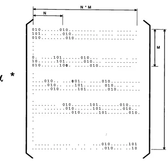
n-*

A

two-dimensional

image

x of

size

N

by

M

can represented

by

a

one-dimensional

vector of

size

NM

by

lexicographic

ordering.

The

prediction operator

P is

represented

by

a square

matrix with

dimension NM

x

NM. The

matrix

P

shown

in Figure

4-4

is

the

result of a

fourth-order

predictor

from Figure 1-1

where

the

elements

B, D,

E

and

G have the

value a and all other elements

have

the

value

0. Note

that

all nonzero

coefficients are

in

a

band

around

the

diagonal

of

the

matrix.

The

zero values shown

in

bold

are

the

result of

the

boundary

condition

that

all pixels

surrounding

the

image

are

zero.

The

norm of

the

matrix

P

can

be

taken

as

the

L_

norm,

the

maximum value of

the

sum of

the

absolute values of

the

coefficients on each row:

Norm(P)

SI P II

=

maxrow

__

|prow,col|

(4-1

9)

col

In

this

case of

fourth-order

predictor

the

norm of

the

matrix

is

4a

.

This is because

each

predictorcaused one of

the

coefficients

in

each row

to

be

unity.

There

are

thus

4

ones

in

each row.

The

norm

is

thus the

sum of

the

absolute values of

the

predictor

coefficients.

For the

general

case,

any

predictor

P that

satisfies

(4-20)

is

a valid predictor.

for

all

rows

col

(4-20)

P

=

a

A

N * M N 010 101 010

010. . . 010. . . 010

0 101 010...

10 101 010..

010 100 010

010. . . 010. . . . 010

-.001 010...

...101 010..

....101 010

N

010 101 010....

.010 101 010..

...010 101 010.

010.. . . 010. .

[image:39.521.100.432.168.488.2]

101 . 10

\

N * M

s

4.2

Constrained

Iterative

Reconstruction

Algorithm

In

some

cases,

a priori

information

about

the

image

to

be

decoded may

be

used

to

advantage

in the

decoding

process.

Usually,

the

image is known

to

be

zero

outside

its

boundaries,

and also

that the

values

of

the

pixels

inside

the

boundaries

may

be known

to

lie in

a certain

range.

These

nonlinear conditions

may

be incorporated in

constraints

that

are

can

be

used

in

the

decoding

process

[19].

If the

image

to

be decoded is

represented

by

x, the

predictor

by

P,

and

the

residual

by

r,

we can write

r=

(I-P)Cx

(4-21)

where

I is the

identity

operator.

The

constraint operator

C

can

be

used

to

enforce

some

boundary

condition on

the

image,

eg., the

image is

always positive within

some

defined

region and zerooutside.

For

all allowed

images

x:

x =

Cx

(4-22)

To

obtainan

iteration

equation,

we can

combine

(4-21)

and

(4-22)

to

obtain

the

identity:

x =

Cx +A(r-(I-P)Cx)

(4-23)

This

equation

is in

the

form

where

the

operator

F

is defined

by

Fx

=

Ar+Cx-A(I-P)Cx

=

Ar

+

Gx

(4-25)

with

G

=

{I-X{I-P))C

(4-26)

The

signal x

that

satisfies

(4-24)

is

called a

"fixed

point

of

the

transformation

F". A

standard method

for

finding

such

solutions

is the

method

of

successive approximations

based

upon

the iteration

equation

xk+1=Fxk=Ar

+

Gxk

(4-27)

The

parameter

X

can

be

used

to

control

the

rate

of

convergence

of

the iteration.

Any

valid

image

can

be

chosen

for the initial image

Xn.

Often the

null

image is

chosen as a

matter of convenience.

Note

that

when

the

explicit constraint

C is

removed

and

X is

chosen

as

1

, equation

(4-27)

becomes

the

same

as

equation

(4-2).

4.2.1 Convergence

It is

assumed

that the

images

x

and

the

outputs of

the iteration

xk

are members

of

a

complete normed

linear

vectorspace,

with norm

llxll

defined,

for

example,

by

H-"=|

[allpixels

__X|2|

(4-28)

Suppose

that

Fxs-FXj\\<y\\xs-Xj

(4-29)

In the

range

0

<

y

<

1,

the

operator

F is

said

to

be

a

"contraction

mapping"

[19]. If

y

=1

the

operator

F is

said

to

be

nonexpansive.

If

y

=

1

_and

(4-29)

holds only

if

X|=Xj

then the

operator

F is

strictly

nonexpansive.

The

term

IIjc,-jc;II

can

be interpreted

as

the

distance

between two

images,

Xj

and

Xj.

A

contraction

mapping

has the

property

of

reducing

the

distance between

images,

as

illustrated in Figure 4-5.

Figure 4-5 Contraction mapping

If

the

operator

F

is

acontraction

mapping

then

it has

a unique

fixed

point xsuch

that

x=Fx.

Every

sequence

defined

by

the iteration

converges

to

x

for

every

choice of

A

consequence

_of

(4-29)

is

\\x-xk\\<-

\\x-x0\\

(4-30)

\-y

Thus,

every

sequence

of

iterations

converges

geometrically

to the

_unique

fixed

_pointx

in the

sense

that

lim^^

II x-xk

11=

₀

.

From

above

it

also

follows

that

II

Fx{

-FXj

INI

Gxi

-Gxj

II

(4-31

)

If F is

a contraction operator

then

G

is

a contraction

operator,

and

the

iteration

will

thus

converge

with

either

F

or

G

being

a contraction operator.

The

convergence properties

can

be

controlled

by

the

choice

of

the

parameter

X

in

(4-25).

By

making

X

sufficiently

small

it is

always

possible

to

ensure

that

F is

a

contraction mapping.

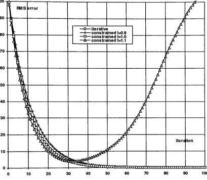
As

an

illustration

of

the

behavior

of

the

convergence

process as a

function

of

X,

the

image

"Lena"

was

coded

using

this

process.

The difference between

the decoded image

and

the

original

image

as a

function

of

the

iteration

number

is

shown

in

Figure 4-6 for three

values of

X:

0.9, 1.0,

and

1.1. The

constrained

iteration

with

X

=

1

.0

behaves exactly

as

the

standard

iteration

process

discussed

above.

The

process with

X

=

1.1

converges

at

first but

starts

to

diverge

after

about

40

iterations.

100

90

80

70

60

50

40

30

20

10

T

RMS

srror

0 iterative

Ined 1=0.9 a constrained1=1.0

A constrained1=1.1

iteration

- iiinrnnOJULLrrrmin 1 1 1 1 1 11"mi ii ii

[image:44.521.57.466.98.454.2]

10 20 30 40

4.3

Direct

Decoding

Sometimes

it is

preferable

to

use

a

one-step

decoding

process

instead

of

the iterative

solution

described before. This may be

due to

computational

limitations

_such

as speed

or

storage requirements.

The

one-step

process

may

be faster

to

compute

than the

iterative

process.

For

large images memory

required

to

store

the

whole

image

may

be

a

problem.

However,

the

direct

method can

be

implemented

efficiently

in

a

way

that

only

part of

the

image

is

needed

in

memory

at

any

time.

If the

estimation

operator

P is line