http://dx.doi.org/10.4236/am.2014.55078
The Construction of Locally D-Optimal
Designs by Canonical Forms to an
Extension for the Logistic Model
Irene García Camacha Gutiérrez, Raúl Martín Martín
Mathematics Department, Castilla-La Mancha University, Toledo, Spain Email: [email protected], [email protected]Received 8 December 2013; revised 8 January 2014; accepted 15 January 2014
Copyright © 2014 by authors and Scientific Research Publishing Inc.
This work is licensed under the Creative Commons Attribution International License (CC BY). http://creativecommons.org/licenses/by/4.0/
Abstract
Logistic regression models for binary response problems are present in a wide variety of industri-al, biologicindustri-al, social and medical experiments; therefore, optimum designs are a valuable tool for experimenters, leading to estimators of parameters with minimum variance. Our interest in this contribution is to provide explicit formulae for the D-optimal designs as a function of the unknown parameters for the logistic model log
(
η(
x,θ)
(
1−η(
x,θ)
)
)
= +α βx+δq where q is an indicatorvariable. We have considered an experiment based on the dose-response to a fly insecticide in which males and females respond in different ways, proposed in Atkinson et al. (1995) [1]. To find the D-optimal designs, this problem has been reduced to a canonical form.
Keywords
Binomial Response; D-Optimal Design; Canonical Form
1. Introduction
with success probability 1
2. The theory of optimal design is used to calculate the optimal dose levels with a determinate probability of death.
To model the experiment, the logistic model for binary data was chosen. Denoting η as the probability of death, x as the logarithm of dose (in micrograms per millilitre) and y as the number of deaths, it must be:
( )
( )
e * *| 1, with , , ,
1 e x q
x q
y x Bi x a x b
α β δ
α β δ
η η θ = ++++ ≤ ≤
+
where q is a factor with values 0 for males and 1 for females and being θ=
(
α β δ, ,)
the unknown parameters vector. This model can be linearized by the logarithm of the probability ratio: log(
η
(
1−η
)
)
= +α β
x+δ
q=µ
Atkinson et al. (1995) [1]. A wide range of dichotomous response-mechanisms can be expressed in terms of the previous model.2. Optimum Design
The main objective of optimal experimental design is to select where and how many trials are necessary to be collected in order to achieve an optimal estimation of the model parameters. The observations will be taken into experimental region, χ , which will be in most cases a closed interval of the real line, a b*, *. On χ it is defined an approximated design as
1 2
1 2
, n
n
x x x
p p p
ξ =
where pi denotes a probability measure with support on x1,,xn. The number of support points is guaranteed to be finite, or at least it is possible to find one finite equivalent, as consequence of Caratheodory’s theorem. Due to the continuity of probability measure chosen, it may occur not to obtain an exact number of trials for each dose level. However, the theory assures us that when the number of observations is sizeable, the integer approximation of the values is enough good.
To proceed with this type of problems, a certain functional from the called Fisher information matrix is required to achieve its maximum value. According to the considered model, it is built the information matrix to a single observation x on an insect of known sex as
( )
( )
, , , ,
i j
i j
M xθ ω xθ µ µ
θ θ ∂ ∂ =
∂ ∂
being ω
(
x,θ)
=λ(
x,θ)
=η(
1−η)
the variance used in fitting a generalized model by weighted least squares (McCullagh and Nelder, 1989 [2]). Nevertheless, the matrix just defined does not take into account the differences on the response previously mentioned. In spite of the experimental limitations about the lack of sex knowledge, it is possible to modify the above matrix to consider this uncertainly as it is shown:( )
( )
( )
2
2 2
1 1 0
, 0.5 , 0.5 , 0 .
1 1 0 0 0
M F
x x x
M x x x x x x x x
x
θ ω θ ω θ
= +
In this work, the function of the information matrix chosen is D-optimality criteria. This criterion minimizes the volume of the confidence ellipsoid of the parameters and it is given by
φ
DM( )
ξ θ
, = M( )
ξ θ
, or equivalently logM( )
ξ θ
, which has the advantage of being a concave function. This optimality criterion has received much attention in the literature because of its direct interpretation (Silvey, 1980 [3]).3. Canonical Forms
problem is transformed through a suitable choice from χ to Z , the dependence of the optimal design on the true value of θ for given design space χ will be replaced, in the transformed problem for arbitrary Z, which will vary with θ. Then, if we are able to solve the transformed problem, we have implicitly solved the original design problem (Ford et al. (1992) [4]). The invariance of the design criteria chosen by the trans- formation is an indispensable requirement for performing this canonical version of the problem.
First, we consider the chosen model as a distribution function which is denoted by η θ
(
,x)
=F(
α β+ x+qδ)
. Let’s suppose the insect sex is known. The following argument is valid for both males and females, so we will denote with the factor q an individual regardless of gender. Applying the change of variable z= +α β
x, the original problem can be reformulated as(
)
e, , 1 e z q z q z δ δ
η θ′ = ++
+
with * *
a z b
α β+ ≤ ≤ +α β or * *
a z b
α β+ ≥ ≥ +α β depending on
β
’s sign. The information matrix can bebuilt using the chain's rule for n dose levels as below:
( )
( ) ( )
(
)
(
(
)
)
(
)
(
)
( ) ( )
1 1 1 1 1 1 , t ni i i x
i i i
n n
t i i i i i i i
i i
p H x H x M
F z q F z q
p z q x x q p v x v x
q ξ δ δ ω δ = = = = + − + = + =
∑
∑
∑
being( )
(
(
)
)
(
)
,(
(
)
)
(
)
,(
(
)
)
(
)
ti i i i i i
i
i i i
F z q z q F z q z q F z q z q
H x
z q z q z q
δ δ δ δ δ δ
δ α δ β δ δ
∂ + ∂ + ∂ + ∂ + ∂ + ∂ +
= ∂ + ∂ ∂ + ∂ ∂ + ∂
the partial-derivative vector from the chain's rule, f the probability density function and
( )
i(
i)(
1 i)
tv x = ω z +qδ x q . Note we have defined
(
)
(
(
)
(
(
)
2)
)
1 i i
i i
f z q
z q
F z q F z q
δ ω δ δ δ + + = + − +
abusing notation. The previous transformation can be expressed in matrix form as
1 1 0 0 1 1
0 ,
0 0 1
z x B x
q q q
α β = = and defining,
( )
( )
(
)
(
)
(
(
)
)
(
)
(
)
(
(
)
)
1 0 0 1 0
1 0 0 1
1 , 1 i i i i i i
g z Bv x
f z q
x
F z q F z q q
f z q
z
F z q F z q q
δ α β δ δ δ δ δ = + = + − + + = + − +
the partial-derivative vector v x
( )
can be expressed in terms of z through v x( )
=B g z−1( )
since B is in- vertible for beingβ
≠0. Let us write the information matrix using the formula for change of basis as( )
1( )
x z
transformations of the design space, the maximization problem of Mx
( )
ξ determinant reduces to maximize( )
z
M ξ . Hereafter, it will only work with the information matrix depending on z and then it will carry the inverse change out for solving the original problem without loss of concept. Note the parameter dependence has been considerably reduced:
( )
(
)
(
)
( ) ( )
1 1 1 . n n tz i i i i i i i
i i i
M p z q z z q p g z g z
q
ξ ω δ
= = = + =
∑
∑
By adding uncertainty about sex, the information matrix to the design 1 2
1 2
n
n
z z z
p p p
ξ =
with
1 1
n i i=p =
∑
for n dose levels results( )
( ) ( )
( ) ( )
1
0.5 n
t t
z i F i i M i i
i
M ξ p g z g z g z h z
= =
∑
+ being,( )
(
)
(
)
(
)
ii i i F
i
z
g z z z
z ω δ ω δ ω δ + = + +
and
( )
( )
( )
. 0i
i i i M
z
g z z z
ω ω =
The above expression can be reformulated into a more general formula
( )
2( ) ( )
1
0.5 ,
n
t
z i i i
i
M ξ p g z g z
=
=
∑
(1)where the zi’s are repeated to consider the information by each possibility about sex since their partial derivatives are different. The novelty of this paper is described in the previous lines. The simplified formulation of the information matrix will allow us to achieve analytical expressions for the optimal weights for several cases in the next section.
4. Results
The aim of our study is to select where and how many observations must be collected in order to reduce the volume of confidence ellipsoid of the parameters as possible. For this purpose, it is necessary to obtain an expression of the determinant of the information matrix which will be maximized later. To calculate the determinant to the information matrix written as (1), it is possible to apply the following formula to its explicit expression given by Ardanuy et al. (1999) [6]:
( )
( ) ( )
1{
( )
}
1 2 2 1 , m j m n
z i i i i i k i
i i i
M ξ p g z g z p p g z
= < <
=
∑
=∑
⋅
(2) being m the number of parameters and ij the elements of S2n, the symmetrical group of 2n-order permutations. We focus the study to calculate optimal designs to a small size of observations, two and three design points. The reason for this choice is that the upper and lower bound for the number of point suffers a slight modification due to each trial has two reading. Then the system will be non-singular if there are at least
1 2
m+
point since m is odd and the Caratheodory upper's bound will be halved with
(
1)
4m m+
. The only possibilities are the considered in the present work.
4.1. Two Points Design
( )
(
)
(
)
( )
(
)
(
)
( )
(
)
(
)
(
)
(
)
(
)
( )
( )
(
)
( )
( )
(
)
(
)
(
)
(
)
( )
(
)
(
)
( )
(
)
(
)
(
)
( )
(
)
( )
( )
(
)
( )
(
)
21 1 2
2
1 1 1 1 2 2
1 2
2
1 1 2
2
1 1 1 1 2 2
1
2
1 2 2
2
1 1 2 2 2 2
1 2
2
1 2 2
2
1 1 2 2 2 2
2 0.5 1 0 1 0 0 1 0 1 0 0 z
z z z
M p p z z z z z z
z z
z z z
p p z z z z z z
z
z z z
p p z z z z z z
z z
z z z
p p z z z z z z
z
ω δ ω ω δ
ξ ω δ ω ω δ
ω δ ω δ
ω δ ω ω
ω δ ω ω
ω δ
ω δ ω δ ω
ω δ ω δ ω
ω δ ω δ
ω ω δ ω
ω ω δ ω
ω δ + + = − + + + + + + − + + + + + − + + + + + + − + +
(
)(
)
(
) (
)
(
)
(
)
2 2 2 20.5 1 1
0.5 1 1 ,
p p A B p p C D
p p E p p F
= − + + − + = − + − (3)
where E and F are the squares of the determinants which result from combining the column matrices
( )
i ,( )
iF F
g z g z with i=1, 2 and operating conveniently. An analytical expression to the optimal weights can be obtained calculating the critical points for the last expression:
( )
(
)
(
)
(
)
2 2
2 * 2
3 2 2 0 .
3 z
M F E F EF E
F E p E F p F p
p F E
ξ
∂ − ± − +
= − + − + = ⇒ =
∂ −
To compute the optimal points z z1, 2 will be enough to replace *
p in the determinant expression and to use a maximization routine. Note the parameter dependence still persists due to non-linearity of the model. To avoid such dependence, Chernoff (1953) [7] suggests providing a prior guess for the parameters θ0 =
(
α β δ0, 0, 0)
. In that sense, the achieved designs in the present work will be called locally D-optimal. The parameter estimates were obtained in Atkinson et al. (1995) [1]. The last step will be to calculate the value of the original variables through inverse change* * 0 0 i i z x α β −
= . The obtained result is shown in Table 1.
4.2. Three Points Design
It is known from other previous works that it can consider a symmetrical design for the present case. Let's us assume such design 1 2 3
1 2
z z z
p p p
ξ =
−
. Applying the determinant formula and proceeding analogously as
(3), it is possible to achieve a tractable expression for the determinant and an analytical formula for the optimal weights in a way:
( )
22 * 3
3 2 0 ,
3 z
M B B AC
Ap Bp C p
being A, B and C the squares of the determinants which result from applying the formula to its fast calculation grouped conveniently. Taking into account the previous considerations, the results are shown in Table 2.
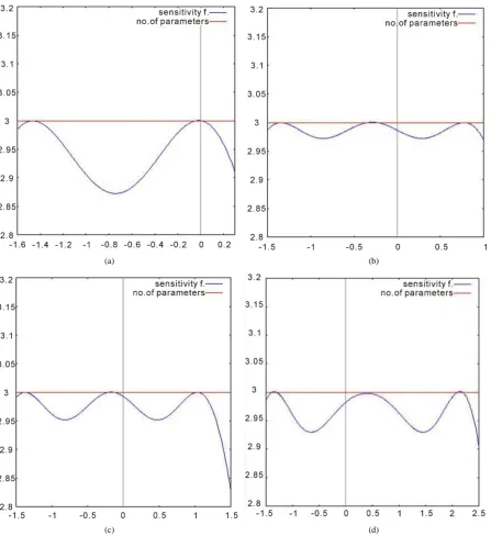
An advantage of working with approximate designs is that the optimality of a design can be easily checked. Kiefer and Wolffowitz (1960) [8] provided a main result for optimal experimental design theory: the general equivalence theorem. The central point of this theorem establishes a necessary condition to check whether a proposed design is D-optimal or not. It consists of verifying if the standardized variance of the prediction, which is known as sensitivity function and is defined as
( )
( )
1( ) ( )
, t ,
d x
ξ
= f x M−ξ
f xis equal to number of parameters in the support points of the design. However, for the present case it is not possible to apply directly the above formula due to lack of knowledge about gender. It requires to use an extension of the equivalence theorem motivated by Chaloner and Larntz (1989) [9]:
( )
*( ) ( )
1( ) ( )
( )
1( ) ( )
, 0.5 M Mt M 0.5 F Ft( ) F .
d x
ξ
= w x f x M−ξ
f x + w x f x M−ξ
f x ≤mThe results shown inFigure 1 allows us to validate the optimal designs proposed in this work. As we can observe from the figures, the points where the sensitivity function intersects the number-parameter line represent the optimal points obtained with the procedure described in this paper.
5. Conclusions
In this paper, it is proposed the use of canonical forms to solve a problem non-standard of optimal experimental designs laid out by Atkinson et al. (1995) [1] upon calculating the optimum dose of a fly insecticide. The main difficulty arises by adding uncertainty about gender since they differ in the response and the experiment only senses applied on the whole population. The witty transformation of the problem to a canonical version reduces the parameter dependence leading to analytical expression of the optimal weights. From these, we are able to compute D-optimal designs for several cases. In particular, it is constructed optimal designs for two and three dose levels.
Regarding future work, we will try to take advantage of the transformation geometry, G Z
( )
, for identifyingTable 1. Locally D-optimal designs for two points design.
0 1.804
α = , β =0 1.1757, γ = −0 1
* i
x −1.757 −0.018
* i
p 0.5 0.5
Table 2. Locally D-optimal designs for three points design.
0 1.804
α = , β =0 1.1757
0 2.599
γ = − *
i
x −1.347 −0.287 0.772
* i
p 0.375 0.250 0.375
0 3
γ = − *
i
x −1.378 −0.173 1.032
* i
p 0.339 0.322 0.339
0 5
γ = − *
i
x −1.349 0.396 2.141
* i
(a) (b)
[image:7.595.92.540.82.571.2](c) (d)
Figure 1. Testing locally D-optimal designs (α0=1.804,β0=1.1757). (a) 2 points: γ = −0 1; (b) 3 points: γ = −0 2.599; (c) 3 points: γ = −0 3; (d) 3 points: γ = −0 5.
the support point. It is known that these are the points of contact between G and the smallest ellipsoid centred on the origin containing G (Sibson, 1972 [10], Silvey and Tittetington, 1973 [11], Silvey, 1980 [3], and Torsney and Musrati, 1993 [12]). However, this procedure must be adapted non-trivially to add two readings by observation with their corresponding probabilities.
References
[2] McCullagh, P. and Nelder,J.A. (1992) Generalized Linear Models. Chapman and Hall, London.
[3] Silvey,S.D. (1980) Optimal Design. Chapman and Hall, London. http://dx.doi.org/10.1007/978-94-009-5912-5 [4] Ford, I., Tosney, B. and Wu,C.F.J. (1992) The Use of a Canonical form in the Construction of Locally Optimal De-
signs for Non-Linear Problems. Journal of the Royal Statistical Society: Series B, 54, 569-583. [5] Fedorov,V.V. (1972) Theory of Optimal Experiments. Academic Press, New York.
[6] Ardanuy, R., Lopez-Fidalgo, J., Laycock, P.J. and Wong,W.K. (1999) When Is an Equally-Weihted Design D-Optimal?
Annals of the Institute of Statistical Mathematics, 51, 531-540. http://dx.doi.org/10.1023/A:1003954207112
[7] Chernoff,H. (1953) Locally Optimal Designs for Estimating Parameters. The Annals of Mathematical Statistics, 24, 586-602. http://dx.doi.org/10.1214/aoms/1177728915
[8] Kiefer, J. and Wolfowitz,J. (1960) The Equivalence of Two Extremun Problems. Canadian Journal of Mathematics, 12, 363-366.
[9] Chaloner, K. and Larntz, K. (1989)Optimal Bayesian Design Applied to Logistic Regression Experiments. Journal of Statistical Planning and Inference, 21, 191-208. http://dx.doi.org/10.1016/0378-3758(89)90004-9
[10] Sibson, R. (1972)Discussion on Results in the Theory and Construction of D-Optimun Experimental Designs (by H. P. Wynn). Journal of the Royal Statistical Society, 34, 174-175.
[11] Silvey, S.D. and Titterington,D.M. (1973) A Geometrical Approach to Optimal Design Theory. Biometrika, 60, 21-32. http://dx.doi.org/10.1093/biomet/60.1.21