http://dx.doi.org/10.4236/jilsa.2014.61004
Constrained Nonlinear Model Predictive Control of a
Polymerization Process via Evolutionary Optimization
Masoud Abbaszadeh
1, Reza Solgi
21
Department of Research and Development, Maplesoft, Waterloo, Canada; 2Swiss Finance Institute, University of Lugano, Lugano, Switzerland.
Email: [email protected], [email protected]
Received April 24th, 2013; revised November 24th, 2013; accepted January 1st, 2014
Copyright © 2014 Masoud Abbaszadeh, Reza Solgi. This is an open access article distributed under the Creative Commons Attribu-tion License, which permits unrestricted use, distribuAttribu-tion, and reproducAttribu-tion in any medium, provided the original work is properly cited. In accordance of the Creative Commons Attribution License all Copyrights © 2014 are reserved for SCIRP and the owner of the intellectual property Masoud Abbaszadeh, Reza Solgi. All Copyright © 2014 are guarded by law and by SCIRP as a guardian.
ABSTRACT
In this work, a nonlinear model predictive controller is developed for a batch polymerization process. The physical model of the process is parameterized along a desired trajectory resulting in a trajectory linearized piecewise model (a multiple linear model bank) and the parameters are identified for an experimental polymeri-zation reactor. Then, a multiple model adaptive predictive controller is designed for thermal trajectory tracking of the MMA polymerization. The input control signal to the process is constrained by the maximum thermal power provided by the heaters. The constrained optimization in the model predictive controller is solved via ge-netic algorithms to minimize a DMC cost function in each sampling interval.
KEYWORDS
Model Predictive Control; Genetic Algorithms; Polymerization; Methyl Methacrylate; Parameter Identification
1. Introduction
Model predictive control (MPC), is a model based on ad- vanced process control (APC) technique that has been proved to be very successful in controlling highly complex dynamic systems. It naturally supports design for MIMO and time-delayed systems as well as state/input/ output constraints. MPC is generally based on online optimization but in the case of unconstrained linear plants, closed form solutions can be derived analytically. However, when there are constraints over the control inputs (i.e. actuators) and/or process states, which is often the case, an online (i.e. real-time) constrained optimization problem has to be solved in each sampling interval, even if the plant model is linear and time invariant. This online optimiza-tion usually requires a high computaoptimiza-tional power; how-ever, since chemical processes are typically of slow dy-namics, such controllers have been designed and imple-mented on various chemical plants with great success.
Moreover, due to recent advancements of computa- tional hardware and software tools, the usage of MPC is rapidly expanding to other control domains including elec-
trical machines, renewable energy, aerospace and auto-motive control systems.
studied an expert neural network as an internal model in control of solution polymerization of vinyl estate. In their study, they compared their neural network control with a classic PID controller. Clarke-Pringle and MacGregor [5] studied the temperature control of a semi-batch industrial reactor. They suggested a coupled non-linear strategy and extended Kalman filter method. Mutha et al. [6] sug-gested a non-linear model based on control strategy, which includes a new estimator as well as Kalman filter. They conducted experiments in a small reactor for solu-tion polymerizasolu-tion of MMA. Rho et al. [7] assumed a first order model plus dead time to pursue the control studies and estimated the parameters of this model by on line ARMAX model. Nonlinear predictive control of the batch reactor considered [8,9] via PCA and Wiener mod-eling approaches, respectively. When MPC is formulated as a state feedback controller, the full state information is required which must be provided using state estimators in nonlinear H2 (e.g. EKF) or nonlinear H∞ paradigms [10-12]. Rafizadeh [13] designed a sequential lineariza-tion adaptive controller for the solulineariza-tion polymerizalineariza-tion of methyl methacrylate in a Batch Reactor.
This paper presents a constrained model predictive control of an MMA reactor, based on the genetic algo-rithm optimization. A previously developed mechanistic model of the process was used. The model is a sequential piecewise linearization along a selected temperature tra-jectory. The piecewise linear model is used both for the plant output calculation through the prediction horizon and for the closed loop simulation of the controller, using a time-triggered switching mechanism. We are using an output feedback MPC, therefore, no state estimator is required, which is advantageous. The results of tracking the trajectory and eliminating noise and disturbances show a promising performance of the controller.
2. Polymerization Mechanism
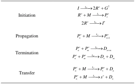
Methyl methacrylate normally is produced by a free radical, chain addition polymerization. Free radical po- lymerization consists of three main reactions: initiation, propagation and termination. Free radicals are formed by the decomposition of initiators. Once formed, these radi-cals propagate by reacting with surrounding monomers to produce long polymer chains; the active site being shifted to the end of the chain when a new monomer is added. During the propagation, millions of monomers are added to P1o radicals. During termination, due to reactions among free radicals, the concentration of radicals decrea- ses. Termination is by combination or disproportionate reactions. With chain transfer reactions to monomer, ini- tiator, solvent, or even polymer, the active free radicals are converted to dead polymer. Table 1 gives the basic
free radical polymerization mechanism [14].
The free radical polymerization rate decreases due to reduction of monomer and initiator concentration. How- ever, due to viscosity increase beyond a certain conver- sion there is a sudden increase in the polymerization rate. This effect is called Trommsdorff, gel, or auto-accelera- tion effect. For bulk polymerization of Methyl Methacry-late beyond the 20% conversion, reaction rate and mo- lecular weight suddenly increase. In high conversion, because of viscosity increase there is a reduction in ter- mination reaction rate.
3. Mathematical Modeling of Polymerization
The polymer production is accomplished by a reduction in volume of the mixture. The volumetric reduction fac- tor is given by:p m
p
ρ
ρ
ε
ρ
−
= (1)
The instantaneous volume of mixture is given by:
(
)
0
1 m M
V εx β
ρ
= − + (2)
The parameter β is defined as:
1 s
s f
f
β =
− (3)
During the free radical polymerization, the cage, glass, and gel effects occur. For the cage effect, the initiator efficiency factor is used. The CCS (Chiu, Carrat and Soong) model is used in this study to take into considera- tion the glass and the gel effects. Therefore, propagation rate constant, kp, is changing according to:
0
0
1 1
p
p p
k k D
λ θ
= + (4)
0 p
[image:2.595.307.541.591.735.2]k is changing as Arrhenius function, and D is given by equation:
Table 1. Polymerization Mechanism. 2
d o
k
I→ R +G↑
1
i
o k o
R +M→P 2Ro→kti I′
Initiation
1
p
k
o o
n n
P +M→P+ Propagation
tc
o o k
n m n m
P +P →D+
td
o o k
n m n m
P +P →D +D Termination
1
f
k
o o
n n
P +M→P +D
s
o k o
n n
P +M→ +s D
(
)
1 exp 1 p p D A B ϕ ϕ − = + − (5)Similarly, termination rate constant, kt, is given by
0
0
1 1
t
t t
k k D
λ θ
= + (6)
0 t
k is changing as Arrhenius function. θp and θt are adjustable parameters related to propagation and ter-mination rate constants, respectively. All other necessary parameters and constants for this model are given in [1, 14,15].
Long Chain Approximation (LCA) and Quasi Steady State Approximation (QSSA) are used in this study. Equ- ations are highly nonlinear and, using Taylor expansion series, these equations were converted to linearized form. The linearized state space form is given by:
0 0 d 0 d 2 j j o po X X i i A P T T t T T m C α = + ′ ′ ′ ′ ′ (7)
[ ]
[ ]
[ ]
1 1 1
2 2 21
3 3
0
0
0 0
s s s
s s s
r r
p p
s s
r o
r
o po o po
f f f
x I T
f f f
x I T
A
UA UA UA
f f
x I mC mC
UA UA
UA
m C m C
∞ ∞ ∂ ∂ ∂ ∂ ∂ ∂ ∂ ∂ ∂ ∂ ∂ ∂ = + ∂ ∂ − ∂ ∂ + −
[
0 0 1 0]
j X i T T T ′ = ′ ′
[image:3.595.66.284.302.586.2]The molecular properties of the produced polymer are controlled by ensuring the reaction temperature is chang- ing according to a desired reference trajectory. This is a tracking control problem which we are solving using MPC.
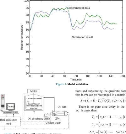
Figure 1 shows the result of model validation [14]. As it is seen, the model is a good representative of the proc-ess. Equation (7) is converted to the transfer function for reaction temperature to input power:
( )
( )
2
3 4 5
4 3 2
1 2 3 4 5
T s n s n s n
P s d s d s d s d s d
′ = + +
+ + + + (8)
The result of sequential linearization is 131 transfer functions along the temperature profile. See [13,14] for a more detailed description of the MMA polymerization dynamic modeling.
4. Experimental Setup
A schematic representation of the experimental batch reactor setup is shown in Figure 2 [14]. The reactor is a Buchi type jacketed, cylindrical glass vessel. A multi- paddle agitator mixes the content. Two Resistance Tem-perature Detectors (RTDs) of PT100 type were used with accuracy of ±0.2˚C to measure the reactor temperature and the oil temperature in the oil bath. Methyl Methacry-late and Toluene were used as monomer and solvent, respectively. Benzoyl Peroxide (BPO) was used as the initiator. The heater, heats the oil circulating the oil bath, which is pumped into the reactor. Cool water is circu-lated in a coolant coil inside the oil bath through an elec-tric on/off valve and acts as a safety feature to prevent the oil and consequently the reactor from overheating. The RTD outputs are converted into 0 - 10 VDC through a bridge and an instrument amplifier and are read by the data acquisition card A/D channels. The controller output is fed into a MOSFET-based power electronics switching circuit as PWM signals. The maximum heater power available is 1000 W, which is a constraint on the control signal.
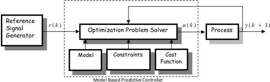
5. Model Predictive Control
Due to its high performance, model predictive control method has received a great deal of attention to control chemical processes, in the last few years. Figure 3 shows block diagram of a model predictive controller.
There are three main approaches to model predictive control, MAC (Model Algorithmic Control), which is based on system’s impulse response, DMC (Dynamic Matrix Control), which uses the process step response samples, and GPC (Generalized Predictive Control), which is based on the process transfer function. In practice, it is easier to obtain step response samples rather than im-pulse response or a full transfer function, and therefore the DMC method is more popular. We use the DMC method in this research. The cost function is defined as:
(
)
(
)
( )
1 1 2 2 1 1 1 0 1000N P M
Q R
i N i
J e t i u t i
u t + = + = = + + ∆ + − ≤ ≤
∑
∑
(9)where P, M and N1 are prediction horizon, control
hori-zon and pure time delay, respectively. Matrices RM M×
and QP P× are weighting matrices used in the weighted
Figure 1. Model validation.
Figure 2. Schematics of the experimental setup.
(
)
(
)
(
)
(
)
(
) (
)
d p
d m
e t i y t i y t i
y t i y t i d t i
+ = + − +
= + − + − + (10)
where yp and ym are the process and model outputs, and d is the difference between the process and model outputs, including noise, disturbance and model mis-match. yd
( )
t is the desired output based on the refer-ence input. If ysp( )
t is the reference input, the follow-ing filtered form is used as the trackfollow-ing trajectory:( )
(
1) (
1) ( )
; 1d d sp
y t =
α
y t− + −α
y t ≤ <α
(11) The parameter α changes the place of the first order smoothing filter pole; the smallerα
the faster output will become. It has been shown that system robustness can be decreased by the reduction ofα
and increment of the manipulated signal [16]. Expanding thesumma-tions and substituting the quadratic forms, the cost func-tion in (9) can be rearranged in a matrix form as
(
) (
T)
Tm D m D
J= Y + −D Y Q Y + −D Y + ∆U R U+ ∆ + (12)
There is no pure time delay in the model, therefore,
1
N is zero, then:
(
)
(
)
T1
m m m
Y =y t+ y t+P (13)
(
)
(
)
T1
D d d
Y =y t+ y t+P (14)
( )
(
)
T1
U+ u t u t M
∆ = ∆ ∆ + − (15)
(
)
(
)
T1
D=d t+ d t+P (16) In forming (14), if the future values of the set point are known, we get
(
)
( ) (
) (
)
(
)
(
) (
) (
)
( ) (
)
(
)
(
)
(
)
( ) (
) (
)
( ) (
)
(
)
2
1
1 1 1
2 1 1 2
1 1 2
1
1
d d sp
d d sp
d sp sp
d d sp
P
P P i
d sp
i
y t y t y t
y t y t y t
y t y t y t
y t P y t y t P
y t y t i
α α
α α
α α α
α α
α α α −
=
+ = + − + + = + + − +
= + − + + +
+ = + − +
= + −
∑
+
which is called programmed MPC. If the future set points are unknown, yd is assumed to be constant dur-ing the prediction horizon, i.e.:
0 20 40 60 80 100 120 140 160
50 55 60 65 70 75 80 85 90 95 100
Time,min
R
eac
tor
t
em
per
at
ur
e
Experimental data
Figure 3. Block diagram of a model predictive controller.
(
1)
(
)
( )
d d d
y t+ ==y t+P =y t
which is called non-programmedMPC. For an LTI sys-tem, without any constraints on output or control signal, the above optimization problem has the following closed form:
(
T)
1 TU+ G QG+ + R − G QE+
∆ = + (17)
where,
D P
E Y Y
∆
= − (18)
1
1
P g
g g
G
g
+
−
=
(19)
And, gi is the step response samples. The matrix G+
is a Toeplitz matrix, containing step response samples as shown in (19). There is no closed form solution for the formulated constrained optimization problem. Hence, an online optimization algorithm (a genetic algorithm) is applied to solve the problem, which will be discussed later. The model output is:
m N N
Y =G+∆U++G−∆U−+g U (20)
1 2 1
2 1
N
N
p
g g g
g g
G
g
−
− −
=
(21)
(
)
(
)
T1 1
U− u t u t N
∆ = ∆ − ∆ − + (22) where N is the number of system step response sam-ples reaching to steady state or equivalent impulse re-sponse steps which lead to zero; and gN is the system DC gain.
(
) (
)
(
)
T1 1
N
U =u t−N u t− +N u t− + −N P (23)
6. The Modified DMC
If the system has any poles close to the origin, the step response will be very slow and the required N is very large. A system including integrator never reaches to the steady state (this case exists in the set of linearized mod-els of the MMA reactor) and N approaches infinity. Hence, instability occurs. This is one of the limitations of the standard DMC formulation, making it only applicable to open loop stable system [17]. To overcome this, one practical solution is as follows. We have
m N N
Y =G+∆U++G−∆U−+g U (24)
Past N N m Past
Y G U g U Y G U Y
∆
− − + +
= ∆ + ⇒ = ∆ + (25)
where YPast is the effect of past inputs on the future system outputs without considering the effect of present and future inputs. Consequently, YPast can be calculated by setting the future ∆us equal to zero and solving the model P steps ahead.
Past
m
U+ Y Y
∆ = → =
As seen in (15) and (19), G+ and ∆U+ are
inde-pendent of N. The only thing determined by N is the dimension of G−, which is omitted now. Therefore,
us-ing this technique, DMC computations become inde-pendent of N. This modified formulation can be used for marginally stable and unstable plants alike.
As discussed in the previous section, we have used a piecewise linear model of the MMA polymerization process. In our application, since the valid model for fu-ture time steps may change through the course of predic-tions, in the computations of YPast, in order to predict the future model outputs, the corresponding valid models are used. In other words, the model used for output predic-tion is scheduled through the prediction horizon, exploit-ing the developed trajectory linearized model. This vir-tual model switching is utilized to calculate the optimal control sequence in each time step. Apparently, another model switching is also applied through the course of time simulation of the closed-loop control system.
Model Cost
Function Constraints
Optimization Problem Solver Process
Reference Signal Generator
Model Based Predictive Controller
) (k
Furthermore, since the whole desired temperature pro-file is known a priori, the programmed MPC is used, utilizing the known future desired temperature trajectory.
7. Genetic Algorithm Optimization
In general, there is no closed form solution for MPC, except the linear time-invariant unconstrained case. Oth-erwise, the optimization problem should be solved nu-merically. If the solution space is convex, sequential quadratic programming techniques (SQP) could be used. Otherwise, either the optimization problem should be a convexified through approximations and relaxation methods or a global optimization algorithm must be used.
Genetic algorithms (GA), are randomized global sear- ching methods developed from the evolution rule in eco-logical world (the genetic mechanism of survival of the fittest). They have internal implicit parallelism and better optimization ability. By the optimization method of prob-ability, they can automatically obtain and instruct the optimized searching space and adjust the searching di-rection autonomously [18].Genetic algorithms, first in-troduced by Holland [19], are robust global random search methods. These methods are founded based on the Dar-winian concept of natural selection and evolution [20], and have been used extensively in optimization and con-trol [21-23].
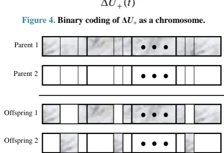
Coding is essential for the GA optimization. Coding is a mapping from solution space to a finite length strings set. Binary coding is the most generally used method. In this method, each point of the solution space is coded as a binary string, which is a permutation of 0 and 1. Each 0 or 1 is called a gene and the string is called a chromo-some. Every potential solution, ∆U+
( )
t , which is a point in the solution space, is coded as a binary word by length of M×Nu. Each element of ∆U+( )
t , is a Nu binary word, called a subchromosome. Figure 4 shows the binary coding of the ∆U+ vector as a chromosome.At the beginning, an initial population that consists of some potential solutions is randomly selected. The final solution is concluded by an iterative method that leads the initial population to an evolutionary one. In each it-eration, the next population is generated by applying the crossover and mutation operators to the selected indi-viduals. Their offspring makes the next population. Their selection probability depends on their fitness function that is a measure of goodness. The encoding method and fitness function definition are the only links between the physical problem and GA optimization. The following fitness function is applied:
(
)
11
F U
J
+
∆ =
+ (26)
1) Encoding
Each element of ∆U+ is assumed as a 12-binary
word. In this way, each chromosome (candidate solution) is a 12×M binary word.
2) Selection
In this stage, pairs of the k-th population, pk, are se-lected to reproduce their offspring. The tournament se-lectionstrategy, which is a stochastic method, is applied to select each parent. In this method, two individuals are randomly selected and their best (according to their fit-ness value) is the winner of the tournament, then, the parents are returned to pk.
3) Crossover
This operator crosses parents to produce the new off-spring by gene interchanging. Crossover may occur in one or more positions in chromosomes. Researchers have suggested several crossover operators such as one point, multipoint and uniform crossover. In this study, a multi-point crossover operator is used to interchange genes between subchromosomes of parents. Figure 5 shows the multipoint crossover genetic operator. The crossover sites are determined randomly.
4) Mutation
In this phase, a random gene from chromosome is se-lected and its value will be changed. To do so, a random number between 0 and 1 is generated and compared with the predetermined mutation probability
(
Pmutation=0.6)
, to see whether the mutation should be done.5) Elitist Strategy
Due to stochastic nature of genetic operators, the best individual of k 1
P + is not essentially better than the k P
one’s. A copy of the best individual of current population is directly transferred to the next one to prevent deterio-ration.
[image:6.595.319.525.522.569.2]The details of optimization algorithm are depicted in
[image:6.595.306.537.562.719.2]Figure 6. In the controller simulation, the optimization is conducted on a population of 50 chromosomes.
Figure 4. Binary coding of ΔU+ as a chromosome.
Figure 5. Multipoint crossover genetic operator.
)
(
t
U
+∆
) (t u
∆ ∆u(t+1) ∆u(t +M −1)
Parent 1
Parent 2
Offspring 1
As mentioned earlier, GA optimization belongs to the family of randomized search algorithms. It is worth men-tioning that, in general, there are no theoretical proofs of the speed of convergence of randomized algorithms (con-vergence within certain time frame, if any). However,
Figure 6. Pseudo-code of the applied GA optimization.
since the cost function is convex and the chemical processes are generally slow, allowing to have sampling periods in the order of tens of seconds, the speed of con-vergence should not be a concern here, provided that the population size and the evolution parameters are selected properly. At the same time, premature convergence is avoided by ensuring good genetic variation. The genetic variation can be regained by using a large enough popu-lation size and also by mutation [24]. On a separate note, in fast systems with millisecond sampling times, the op-timization algorithm may not converge within the sam-pling interval and the optimization computation might be halted. In such cases, especially in mission-critical and safety-critical applications, hybrid algorithms must be utilized using FSQP (Feasible SQP) solvers, to ensure feasibility (satisfaction of all constraints) of the optimizer, in each and every iteration even before convergence.
8. Simulation Results
The population is the foundation of evolution of a genetic algorithm. The character of the population decides the search capability of the genetic algorithm. The astrin-gency of the genetic algorithm is determined by the as-tringency of the population [25].
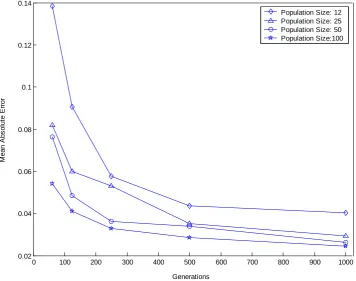
First, the effects of population size and the number of generations on controller performance are studied. As it is shown in the Figure 7, after some thresholds of popu-lation size and number of generations, there is no signif-
Figure 7. Effect of the number of generations and population size on controller performance.
0 100 200 300 400 500 600 700 800 900 1000 0.02
0.04 0.06 0.08 0.1 0.12 0.14
Generations
M
ean A
bs
ol
ut
e E
rr
or
[image:7.595.122.479.439.720.2]icant improvement in controller performance, in com-parison with the great growth deal of computations. The figure exhibits convergence of the GA-based optimiza-tion. The sampling period is 30 seconds and other pa-rameters are as follows:
3 3 3 3
3, , 0.05 , 0.1, u 12
P=M = Q=I× R= ×I× α= N =
[image:8.595.88.514.375.713.2]Our several simulations show that the GA optimization algorithm converges well within the selected MPC sam-pling period in all runs.
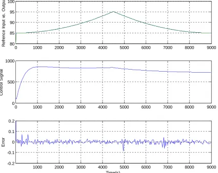
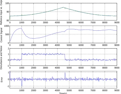
Figure 8 shows the simulation results of controller performance with a population size of 50 and the number of generations equal to 750. The top plot shows the sys-tems output verses the desired thermal trajectory and exhibits controller’s high performance. The middle plot is the control signal, which as seen in the plot, satisfies the constraint. The bottom plot is the tracking error, i.e. the difference between the actual and desired outputs. The DMC controller provides integral action, capable of rejecting step disturbance. The ability of controller to reject noise and disturbance is shown in Figure 9, in which a step output disturbance and a zero mean white Gaussian measurement noise with a variance of 0.1˚C
(STD~0.3˚C) are applied. As seen, the controller has good disturbance rejection performance and the average absolute tracking error is less than 0.25˚C. Compared to the previous results, the adaptive PI control in [13] has a 2˚C average error and the Generalized Takagi-Sugeno- Kang fuzzy controller proposed in [26] has a 1˚C average error; demonstrating the superior performance of the MPC.
9. Conclusion
A sequential piecewise linearized model based predictive controller based on the DMC algorithm was designed to control the temperature of a batch MMA polymerization reactor. Using the mechanistic model of the polymeriza-tion, a transfer function was derived to relate the reactor temperature to the power of the heaters. The coefficients of the transfer function were calculated along the se-lected temperature trajectory by sequential linearization. A genetic algorithm (GA) is applied to the cost function optimization DMC. The simulation result of controller performance shows that the tracking of the profile, noise and disturbances rejection is very good.
Figure 8. The output, control signal and error.
0 1000 2000 3000 4000 5000 6000 7000 8000 9000
80 85 90 95 100
R
ef
renc
e I
nput
v
s
. O
ut
put
0 1000 2000 3000 4000 5000 6000 7000 8000 9000
0 500 1000
C
ont
rol
S
ignal
1000 2000 3000 4000 5000 6000 7000 8000 9000
-0.2 -0.1 0 0.1 0.2
Time(s)
E
rro
Figure 9. The controller performance in the presence of noise and disturbance.
Acknowledgements
The authors would like to thank Dr. Mehdi Rafizadeh for providing the model of the reactor.
REFERENCES
[1] M. Rafizadeh, “Non-Isothermal Modeling of Solution Polymerization of Methyl Methacrylate for Control Pur- poses,” Iranian Polymer Journal, Vol. 10, No. 4, 2001, pp. 251-263.
[2] T. Peterson, E. Hernandez, Y. Arkun and F. J. Schork, “Non-Linear Predictive Control of a Semibatch Polymeri- zation Reactor by an Extended DMC,” American Control Conference, Pittsburgh, 21-23 June 1989, pp. 1534-1539.
[3] M. Soroush and C. Kravaris, “Non-Linear Control of a Batch Polymerization Reactor: An Experimental Study,” AICHE Journal, Vol. 38, No. 9, 1991, pp. 1429-1448. http://dx.doi.org/10.1002/aic.690380914
[4] M. B. De Souza Jr., J. C. Pinto and E. L. Lima, “Control of a Chaotic Polymerization Reactor: A Neural Network Based Model Predictive Approach,” Polymer Engineering & Science, Vol. 36, No. 4, 1996, pp. 448-457.
http://dx.doi.org/10.1002/pen.10431
[5] T. Clarke-Pringle and J. F. MacGregor, “Non-Linear
Adaptive Temperature Control of Multi-Product, Semi- Batch Polymerization Reactors,” Computers & Chemical Engineering, Vol. 21, No. 12, 1997, pp. 1395-1409. http://dx.doi.org/10.1016/S0098-1354(97)00013-6
[6] R. K. Mutha, W. R. Cluett and A. Penlidis, “On-Line Non-Linear Model-Based Estimation and Control of a Polymer Reactor,” AICHE Journal, Vol. 43, No. 11, 1997, pp. 3042-3058. http://dx.doi.org/10.1002/aic.690431116
[7] H. R. Rho, Y. Huh and H. Rhee, “Application of Adap-tive Model-PredicAdap-tive Control to a Batch MMA Polym-erization Reactor,” Chemical Engineering Science, Vol. 53, No. 21, 1998, pp. 3728-3739.
http://dx.doi.org/10.1016/S0009-2509(98)00166-3
[8] J. Flores-Cerrillo, J. F. MacGregor, “Latent Variable MPC for Trajectory Tracking in Batch Processes,” Jour- nal of Process Control, Vol. 15, No. 6, 2005, pp. 651-663. http://dx.doi.org/10.1016/j.jprocont.2005.01.004
[9] G. Shafiee, M. R. Jahed-Motlagh and A. A. Jalali, “Non- linear Predictive Control of a Polymerization Reactor Based on Piecewise Linear Wiener Model,” Chemical Engineering Journal, Vol. 143, No. 1-3, 2008, pp. 282- 292. http://dx.doi.org/10.1016/j.cej.2008.05.013
[10] S. M. Ahn, M. J. Park and H. K. Rhee, “Extended Kal- man Filter-Based Nonlinear Model Predictive Control for a Continuous RIMA Polymerization Reactor,” Industrial
0 1000 2000 3000 4000 5000 6000 7000 8000 9000
80 90 100
R
ef
renc
e I
nput
v
s
. O
ut
put
0 1000 2000 3000 4000 5000 6000 7000 8000 9000
0 500 1000
C
ont
rol
S
ignal
0 1000 2000 3000 4000 5000 6000 7000 8000 9000
-1 0 1 2
D
is
tur
banc
e and N
oi
s
e
1000 2000 3000 4000 5000 6000 7000 8000 9000
-1 0 1
Time(s)
E
rro
& Engineering Chemistry Research, Vol. 38, No. 10, 1999, pp. 3942-3949. http://dx.doi.org/10.1021/ie990240r
[11] M. Abbaszadeh and H. J. Marquez, “Dynamical Robust H∞ Filtering for Nonlinear Uncertain Systems: AnLMI Approach,” Journal of the Franklin Institute, Vol. 347, No. 7, 2010, pp. 1227-1241.
http://dx.doi.org/10.1016/j.jfranklin.2010.05.016
[12] M. Abbaszadeh and H. J. Marquez, “Robust Static Output Feedback Stabilization of Discrete-Time Nonlinear Un- certain Systems with H∞ Performance,” Proceedings of the16th Mediterranean Conference on Control and Auto- mation, Ajaccio, 25-27 June 2008, pp. 226-231
[13] M. Rafizadeh, “Sequential Linearization Adaptive Con- trol of Solution Polymerization of Methyl Methacrylate in a Batch Reactor,” Polymer Reaction Engineering Journal, Vol. 3, No. 10, 2002, pp. 121-133.
http://dx.doi.org/10.1081/PRE-120014692
[14] M. Rafizadeh and M. Abbaszadeh, “Nonlinear Model Predictive Control of Discrete Methyl Methacrylate Po-lymerization for Temperature Profile Tracking,” Amirka- bir Journal of Science and Technology, Vol. 14, No. 55-C, 2003, pp. 811-824.
[15] M. Abbaszadeh, “Nonlinear Multiple Model Predictive Control of Solution Polymerization of Methyl Methacry- late,” Intelligent Control and Automation, Vol. 2, No. 3, 2011, pp. 226-232.
http://dx.doi.org/10.4236/ica.2011.23027
[16] E. F. Camacho and C. Bordons, “Model Predictive Con- trol in the Process Industry,” Springer and Verlag, 1995. http://dx.doi.org/10.1007/978-1-4471-3008-6
[17] P. Lundstorm, J. H. Lee, M. Morari and S. Skogestod, “Limitations of Dynamic Matrix Control”, Computers and Chemical Engineering, Vol. 19, No. 4, 1995, pp. 402-421.
[18] J. Ho, J. Gu, T. Zhao, G. Sun, “A New Resource
Sched-uling Strategy Based on Genetic Algorithm in Cloud Computing Environment,” Journal Of Computers, Vol. 7, No. 1, 2012, pp. 42-52.
[19] J. H. Holland, “Adaptation in Natural and Artificial Sys-tems,” University of Michigan Press, Ann Arbor, 1975.
[20] L. M. Schmitt, “Fundamental Study, Theory of Genetic Algorithms,” Theoretical Computer Science, Vol. 259, No. 1-2, 2001, pp. 1-61.
http://dx.doi.org/10.1016/S0304-3975(00)00406-0
[21] K. S. Tang, K. F. Man, S. Kwong and Q. He, “Genetic Algorithms and Their Applications,” IEEE Signal Proc- essing Magazine, Vol. 13, No. 6, 1996, pp. 22-37. http://dx.doi.org/10.1109/79.543973
[22] R. Bandyopadhyay, U. K. Chakaraborty and D. Patrana- bis, “Autotuning a PID Controller: A Fuzzy-Genetic Ap- proach,” Journal of System Architecture, Vol. 47, No. 7, 2001, pp. 663-673.
http://dx.doi.org/10.1016/S1383-7621(01)00022-4
[23] L. Bernal-Harro, C. Azzaro-Pantel and S. Domenech, “Design of Multipurpose Batch Chemical Plants Using a Genetic Algorithm,” Computers and Chemical Engineer- ing, Vol. 22, Suppl. 1, 1998, pp. S777-S780.
http://dx.doi.org/10.1016/S0098-1354(98)00146-X
[24] Z. Michalewicz, “Genetic Algorithms + Data Structures = Evolution Programs,” 3rd Edition, Springer-Verlag, 1996.
[25] Q. Zhio and L. Xi, “Application of Genetic Algorithm to Huasdorff Measure Estimation”, Proceedings of the 11th International Conference of Knowledge-Based Intelligent Information and Engineering Systems, 2007, pp. 182-189.
![Figure 1 shows the result of model validation [14]. As it is seen, the model is a good representative of the proc-ess](https://thumb-us.123doks.com/thumbv2/123dok_us/7993389.760055/3.595.66.284.302.586/figure-shows-result-model-validation-seen-model-representative.webp)