https://doi.org/10.1007/s00332-017-9433-y
Mean Field Limits for Interacting Diffusions in a
Two-Scale Potential
S. N. Gomes1 · G. A. Pavliotis1
Received: 18 July 2017 / Accepted: 6 December 2017 / Published online: 19 December 2017 © The Author(s) 2017. This article is an open access publication
Abstract In this paper, we study the combined mean field and homogenization limits for a system of weakly interacting diffusions moving in a two-scale, locally periodic confining potential, of the form considered in Duncan et al. (Brownian motion in an N-scale periodic potential, arXiv:1605.05854, 2016b). We show that, although the mean field and homogenization limits commute for finite times, they do not, in general, commute in the long time limit. In particular, the bifurcation diagrams for the stationary states can be different depending on the order with which we take the two limits. Furthermore, we construct the bifurcation diagram for the stationary McKean– Vlasov equation in a two-scale potential, before passing to the homogenization limit, and we analyze the effect of the multiple local minima in the confining potential on the number and the stability of stationary solutions.
Keywords McKean–Vlasov equation·Interacting particles·Multiscale diffusions· Bifurcation diagram·Phase transitions·Desai–Zwanzig model·Curie–Weiss model
Mathematics Subject Classification 35Q70·35Q83·35Q84·82B26·82B80
1 Introduction
Systems of interacting particles, possibly subject to thermal noise, arise in several applications, ranging from standard ones such as plasma physics and galactic
dynam-Communicated by Charles R. Doering.
B
G. A. Pavliotisics (Binney and Tremaine 2008) to dynamical density functional theory (Goddard et al.2012a,b), mathematical biology (Farkhooi and Stannat2017; Lu´con and Stannat
2016) and even in mathematical models in the social sciences (Garnier et al.2017; Motsch and Tadmor2014). As examples of models of interacting “agents” in a noisy environment that appear in the social sciences—which has been the main motivation for this work—we mention the modeling of cooperative behavior (Dawson1983), risk management (Garnier et al.2013) and opinion formation (Garnier et al.2017). Another recent application that has motivated this work is that of global optimization (Pinnau et al.2017).
In this work, we will consider a system of interacting particles in one dimension, moving in a confining potential, that interact through their mean, i.e., a Curie–Weiss type interaction (Dawson1983):
dXti =
⎛
⎝−V(Xit)−θ
⎛ ⎝Xit − 1
N
N
j=1 Xtj
⎞ ⎠ ⎞ ⎠dt+
2β−1dBi
t. (1.1)
Herext := {Xti}iN=1denotes the position of the interacting agents,V(·)a confining potential,θthe strength of the interaction between the agents,{Bti}iN=1standard inde-pendent one-dimensional Brownian motions andβthe inverse temperature. The total energy (Hamiltonian) of the system of interacting diffusions (1.1) is
WN(x)= N
=1
V(X)+ θ 4N
N
n=1
N
=1
(Xn−X)2. (1.2)
Passing rigorously to the mean field limit asN → ∞using, for example, martingale techniques (Dawson1983; Gärtner1988; Oelschläger1984), and under appropriate assumptions on the confining potential and on the initial conditions (propagation of chaos), is a well-studied problem. Formally, using the law of large numbers we deduce that
lim
N→+∞
1 N
N
j=1
Xtj =Ext,
where the expectation is taken with respect to the “1-particle” distribution function p(x,t).1 Passing, formally, to the limit as N → ∞ in the stochastic differential equation (1.1), we obtain the McKean SDE
dxt = −V(xt)dt−θ(xt−Ext)dt+
2β−1dB
t. (1.3)
1 This corresponds to the mean field ansatz for theN-particle distribution function,p
N(x1, . . .xN,t)=
N
The Fokker–Planck equation corresponding to this SDE is the McKean–Vlasov equa-tion (Frank2005; McKean1966, 1967)
∂p
∂t =
∂
∂x V
(x)p+θ x−
Rx p(x,t)dx
p+β−1∂p
∂x
. (1.4)
The McKean–Vlasov equation is a nonlinear, nonlocal Fokker–Planck type equation that we will sometimes refer to as the McKean–Vlasov–Fokker–Planck equation. It is a gradient flow, with respect to the Wasserstein metric, for the free energy functional
F[ρ] =β−1
ρlnρdx+
Vρdx+θ
2 F(x−y)ρ(x)ρ(y)dxdy, (1.5)
where we write the interaction potential asF(x)=12x2. Background material on the McKean–Vlasov equation can be found in, e.g., Carrillo et al. (2006), Frank (2005) and Villani (2003).
The finite-dimensional dynamics (1.1) has a unique invariant measure. Indeed, the processxt defined in (1.1) withV being a confining potential is always ergodic, and
in fact reversible, with respect to the Gibbs measure (Pavliotis2014, Ch. 4),
μN(dx)=
1 ZN
e−βWN(x1,...xN)dx1. . .dxN, Z
N=
RNe
−βWN(x1,...xN)dx1. . .dxN (1.6) whereWN(·)is given by (1.2).
On the other hand, the McKean dynamics (1.3) and the corresponding McKean– Vlasov–Fokker–Planck equation (1.4) can have more than one invariant measures, for nonconvex confining potentials and at sufficiently low temperatures (Dawson1983; Tamura1984). This is not surprising, since the McKean–Vlasov equation is a nonlinear, nonlocal PDE and the standard uniqueness of solutions for the linear (stationary) Fokker–Planck equation does not apply (Bogachev et al.2015).
The density of the invariant measure(s) for the McKean dynamics (1.3) satisfies the stationary nonlinear Fokker–Planck equation
∂
∂x V
(x)p
∞+θ x−
Rx p∞(x)dx
p∞+β−1∂p∞
∂x
=0. (1.7)
Based on earlier work (Dawson1983; Tamura1984), it is by now well understood that the number of invariant measures, i.e., the number of solutions to (1.7), is related to the number of metastable states (local minima) of the confining potential—see Tugaut (2014) and the references therein.
For the Curie–Weiss (i.e., quadratic) interaction potential a one-parameter family of solutions to the stationary McKean–Vlasov equation (1.7) can be obtained:
p∞(x;θ, β,m)= 1
Z(θ, β;m)e
−βV(x)+θ12x2−xm
, (1.8a)
Z(θ, β;m)=
Re
−βV(x)+θ12x2−xm
-2 -1 0 1 2
-2 -1 0 1 2 0 10 20 30 40 50
-1 -0.5 0 0.5 1
[image:4.439.53.385.49.209.2](a) (b)
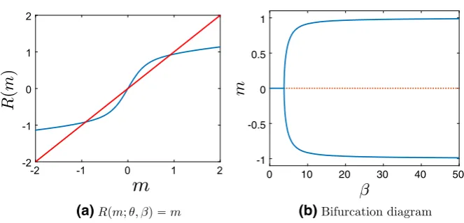
Fig. 1 aPlot ofR(m;θ, β)and of the straight liney=xforθ=0.5,β=10, andbbifurcation diagram ofmas a function ofβforθ=0.5 for the bistable potentialV(x)= x44 −x22 and interaction potential
F(x)= x22
This one-parameter family of probability densities is subject, of course, to the con-straint that it provides us with the correct formula for the first moment:
m=
Rx p∞(x;θ, β,m)dx=:R(m;θ, β). (1.9)
We will refer to this as theself-consistencyequation and it will be the main object of study of this paper. Once a solution to (1.9) has been obtained, substitution back into (1.8) yields a formula for the invariant densityp∞(x;θ, β,m).
Clearly, the number of invariant measures of the McKean–Vlasov dynamics is determined by the number of solutions to the self-consistency equation (1.9). It is well known and not difficult to prove that for symmetric nonconvex confining potentials a unique invariant measure exists at sufficiently high temperatures, whereas more than one invariant measure exists below a critical temperatureβc−1 (Dawson1983,
Thm. 3.3.2; Tamura1984, Thm. 4.1, Thm. 4.2); see also Shiino (1987). In particular, for symmetric potentials,m=0 is always a solution to the self-consistency equation (1.9). Aboveβc, i.e., at sufficiently low temperatures, the zero solution loses stability and
a new branch bifurcates from them =0 solution (Shiino1987). This second-order phase transition is similar to the one familiar from the theory of magnetization and the study of the Ising model. In Fig.1, we present the solution to the self-consistency equation and the bifurcation diagram for stationary solutions of the McKean–Vlasov equation for the standard bistable—Landau—potentialV(x)=x44 −x22.
To compute the critical temperature, we need to solve the equation obtained by differentiating the self-consistency equation with respect to the order parametermat m=0 (see Shiino1987; Frank2005, Sec 5.1.3 for more details):
Varp∞(x) m=0:=
x2p∞(x;β, θ,m=0)dx− x p∞(x;β, θ,m=0)dx)
2
The number of times thatm and R(m;θ, β) cross, i.e., the number of stationary measures, depends on the slope ofR(m;θ, β)at the origin. This is given precisely by Eq. (1.10).
The main purpose of this paper is to study the dynamics and, in particular, bifurca-tions and phase transibifurca-tions for a system of interacting diffusions moving in a rugged energy landscape, coupled through the Curie–Weiss interaction. We are particularly interested in understanding the combined effect of the presence of several local min-ima (metastable states) in the confining potential and of the passage to the mean field limit. We will study the problem for a system of interacting diffusions of the form (1.1) moving in a two-scale, locally periodic confining potential
V(x)=V
x,x
, (1.11)
whereV : (x,y)∈R×Y→R,Ydenotes a periodic box inRd,Y= [0,L]d: V(x,y+k Lei)=V(x,y), k∈Z, (1.12)
and{e1, . . . ,ed}is the canonical basis ofRd. Throughout this paper,L = 2π. The
particles{Xti,i = 1, . . . ,N}are interacting through the Curie–Weiss interaction,
F(x)= x22. This class of potentials provides us with a natural testbed for testing several techniques and methodologies for the study of multiscale diffusions such as maximum likelihood estimation (Papavasiliou et al.2009; Pavliotis and Stuart2007), particle filters and filtering (Imkeller et al.2013; Papavasiliou2007), importance sampling and large deviations (Spiliopoulos2013) and optimal control (Hartmann et al.2014). Of particular relevance to us is the multiscale analysis presented in Duncan et al. (2016a), Duncan et al. (2016b).2In these works, the homogenized SDE for a Brownian particle moving in a two-scale potential inRdvalid in the limit of infinite scale sepa-ration→0 was obtained and the effect of the multiscale structure on noise-induced transitions was investigated. It was shown, in particular, that the homogenized SDE is characterized by multiplicative noise. For a single Brownian particle inRdmoving in a two-scale potential (1.11) (or, equivalently, for a system ofdnoninteracting Brownian particles in a two-scale potential), the homogenized equation reads
dXt = −M(Xt)∇ (Xt)dt+β−1(∇ ·M)(Xt)dt+
2β−1M(X
t)dBt, (1.13)
whereM(·)denotes the diffusion tensor and (·)the free energy—see Sect.2. It is important to note that, in addition to the presence of multiplicative noise, the poten-tial energy driving the dynamics is not simply the average of the two-scale potenpoten-tial over its period, but, rather, the free energy = −β−1lne−βV(x,y)dy. Since
the dynamics (1.13) is finite-dimensional, no phase transitions can occur. In fact, the
2 In fact, in these papers a potential withNmicroscales and one macroscopic scale of the formV(x)= V
x,x,x2, . . .xN
-1 0 1 2 3 4 5
-2 -1 0 1 2 -1 -2 -1 0 1 2
0 1 2 3 4 5
(a) (b)
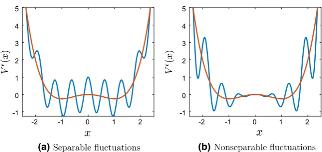
Fig. 2 Bistable potential with (left) separable and (right) nonseparable fluctuations
homogenized dynamics is reversible with respect to the thermodynamically consis-tent Gibbs measure; see the discussion in Sect. 2. It is well known, however, that multiplicative noise can lead to noise-induced transitions, i.e., to changes in the topo-logical structure of the invariant measure (Horsthemke and Lefever1984; Pavliotis
2014, Sec. 5.4). Such phenomena, including multiscale-induced hysteresis effects, for a one-dimensional Brownian particle moving in a multiscale potential, were studied in detail in Duncan et al. (2016a).
Our goal is to study mean field limits for multiscale interacting diffusions of the form
dX,t i = −∇V(Xt,i)dt−
θ
N
N
j=1
∇F(Xt,i−X, j t )dt+
2β−1dBi
t, (1.14)
where the two-scale potential is given by (1.11). The interaction potential F(·)is assumed to be a smooth even function, with F(0) = 0 and F(0) = 0. All of the numerical experiments that we will present will be for the Curie–Weiss quadratic interaction potentialF(x)= 12x2.
The main issues that we address in this work are:
1. What is the effect of the presence of (infinitely) many local minima in the locally periodic confining potential on the bifurcation diagram? In other words, how do the bifurcation diagrams for1 but finite and→0 differ?
2. Do the homogenization and mean field limits commute, in particular when also passing to the long time limitT → +∞? In other words: are the bifurcations diagrams corresponding to theN → ∞, T → ∞, → 0 and → 0, N → ∞,T → ∞limits the same?
[image:6.439.53.386.51.208.2]V(x)= x 4 4 −
x2 2 +δcos
x
and V(x)= x 4 4 −
1−δcos
x
x2 2 . (1.15)
It should be clear from these two figures that the homogenization and mean field lim-its, when also combined with the long time limit, do not necessarily commute. First, the homogenization process tends to smooth out local minima and to even “convex-ify” the confining potential—think of a quadratic potential perturbed by fast periodic fluctuations. This implies, in particular, that even though many additional stationary solutions, i.e., branches in the bifurcation diagram may appear for all finite values of, most, if not all, of them may not be present in the bifurcation diagram for the homogenized dynamics. Furthermore, multiplicative/nonseparable fluctuations of the type presented in Fig.2b tend to flatten the potential aroundx =0. As we will see in Sect.4, this phenomenon is very much related to the lack of commutativity of the limitsN → ∞,T → ∞, →0 and→0, N→ ∞, T → ∞.
We will study these problems using a combination of formal multiscale calcula-tions, (some) rigorous analysis and extensive numerical simulations. There are many technical issues that we do not address, such as the rigorous homogenization study of the McKean–Vlasov equation and the rigorous study of bifurcations in the presence of infinitely many local minima. We will address these in future work.
The rest of the paper is organized as follows. In Sect.2, we study the mean field limit for a system of homogenized interacting diffusions, i.e., the first → 0, then N → ∞limit. In Sect.3, we study the homogenization problem for the McKean– Vlasov equation in a two-scale potential. In Sect.4, we present extensive numerical simulations. Section5is reserved for conclusions.
2 Mean Field Limit of the Homogenized Interacting Diffusions: First
→
0, then
N
→ ∞
In this section, we consider the one-dimensional version of the system of SDEs (1.14). We first take the homogenization limit ( → 0) and then the mean field limit (N → ∞). The homogenization theorem for a system of finite-dimensional inter-acting diffusions moving in a two-scale confining potential is presented in Duncan et al. (2016b). The mean field limit of the homogenized SDE system can be obtained by using the results of Gärtner (1988), Oelschläger (1984).
2.1 Homogenization for Finite System of Interacting Diffusions in a Two-Scale Potential
We consider the system of interacting diffusions
dXti = −∂xV(Xti)dt−
θ
N
N
j=1
∂xF(Xit −X j t)dt+
2β−1dBi
where F is a smooth even function with F(0) = 0 and F(0) = 0 and V is a smooth locally periodic potential of the form (2.7). We introduce the notationxt =
(X1t, . . . ,XtN), so that we have
dxt = −∇W(xt)dt+
2β−1dB
t, (2.2)
where
W(x)=
N
=1
V x,x
+ θ 2N
N
n=1
N
=1
F(xn−x).
andBt is a standard Brownian motion inRN. This equation is of the same form as
Duncan et al.2016b, Eq. (1) and Duncan et al. (2016a), Eqn.(1), with V(Xt)replaced
byW(xt).
Since F does not depend on the fast scale, the results of Duncan et al. (2016b) apply directly to (2.2) and we deduce that the sequencextconverges, as→0, to the solution of the homogenized equation
dxt = −
M(xt)∇ N(xt)−β−1∇ ·M(xt)
dt+
2β−1M(x
t)dBt, (2.3)
where
N(x)= −β−1lnZN(x), (2.4)
for
ZN(x)=
Ye
−βWN(x,y)dy, (2.5)
whereWN(x,y)is defined as in Eq. (1.2),
WN(x,y)= N
=1
V(x,y)+ θ 2N
N
n=1
N
=1
F(xn−x). (2.6)
The convergence is in the sense of weak convergence of probability measures, i.e., the law of the processxt converges weakly to the law of the limiting processxt. The
proof of this result, which is quite standard, is based on the application of Itô’s formula to the solution of an appropriate Poisson equation, Eq. (2.12), the decomposition of the rescaled process into a martingale part and a remainder part, and the use of the martingale central limit theorem. The details can be found in Duncan et al. (2016b). It will be useful to decompose the two-scale potential into its large-scale confining part and the modulated, mean-zero, fluctuations:
V(x)=V0(x)+V1
x,x
, V0(x)=
YV(x,y)dy. (2.7)
However, the choice of the weight does not affect our results. See, e.g., the proof of Proposition3.1.
We note that the free energy N is of the form
N(x)=
N
=1
V0(x)+ θ 2N
N
n=1
N
=1
F(xn−x)
+ψ(x), (2.8)
where
ψ(x)= −β−1lnN=1Ye−βV1(x,y)dy
= −β−1N =1ln
Ye−βV1(x,y)dy
. (2.9)
Finally,M:Rd →Rdsym×dis defined by
M(x)= K(x) ZN(x)
, (2.10)
where
K(x)=
Y(I+ ∇y(x,y))e
−βWN(x,y)dy, x∈Rd, (2.11)
and, for fixedx∈Rd,is the unique weak solution inH1(Y)to ∇y·e−βV1(x,y)(I+ ∇y(x,y))
=0, y∈Y, (2.12)
or
N
i=1
∂ ∂yi e−β
V1(x,y) δ
i j+∂ j(x,y)
∂yi
=0, j=1, . . . ,N,
such that the centering condition Y(x,y)e−βV1(x,y)dy = 0, for all x ∈ Rd is satisfied. The proof of uniqueness of centered solutions to this equation is based on the Lax–Milgram lemma and can be found in Duncan and Pavliotis (2016b, Thm. 2.3). To compute the diffusion tensor (see Duncan et al.2016a, Appendix A for a similar computation), we observe that
Mi j(x)=δi j+
1 ZN(x)
×
Y
∂i
∂yj(x,y)e
−βN
=1V0(x)+N=1V1(x,y)+2θNnN=1N=1F(x−xn)
dy
=δi j+
1 ¯ Z(x)
L 0 · · · L 0 ∂i
∂yj(x,y) N
m=1
whereZ(x)is defined in Eq. (2.5) and
¯ Z(x)=
N
m=1
L
0
e−βV1(xm,ym)dym. (2.13)
Since there is no coupling between the different yi components od Eq. (2.12), it follows that(x,y)can be written in the form(x,y)=(φ(x1,y1), φ(x2,y2), . . . ,
φ(xN,yN)), whereφ(x,y)solves
−L0φ(x,y)= −∂ V1
∂y (x,y), L0= −∂yV1∂y+β
−1∂2
y, (2.14)
and thereforei(x,y)=φ(xi,yi)and
∂i
∂yj(x,y)=
∂φ(xi,yi)
∂yj =δi j
∂φ ∂yj(x
i,
yi).
Substituting in (2.13), we obtain
Mi j(x)= =δi j+
1 ¯ Z(x)
L
0 · · ·
L
0
δi j ∂φ
∂yj(x i,
yi)
N
m=1
e−βV1(xm,ym)dym, (2.15)
and the diffusion tensor is diagonal, with
Mii(x)=1+
1
N
m=1
L
0 e−βV1(x m,ym)
dym L
0
∂φ ∂yi(x
i,yi)e−βV1(xi,yi)dyi × L 0 N
m=1,m=i
e−βV1(xm,ym)dym
=1+L 1 0 e−βV1(x
i,yi) dyi
L
0
∂φ ∂yi(x
i,yi)e−βV1(xi,yi)dyi.
As it is well known (Pavliotis and Stuart 2008, Sec 13.6.1), the one-dimensional Poisson equation (2.14) can be solved explicitly, up to quadratures. We can then obtain formulas for the diagonal elementsMii of the diffusion tensorM(x):
M(x)= 1
1
L L
0 e−βV1(x,y)dy 1
L L
0 eβV1(x,y)dy
We can write the system of stochastic differential equations for the homogenized system of interacting particles:
dXti = −
M(Xit)∂xi (X1t, . . .XtN)−β−1M(Xit)
dt+
2β−1M(Xi t)dBti,
(2.17) fori = 1, . . . ,N, whereMis defined in Eq. (2.16), prime denotes differentiation with respect toxand is given by Equations (2.8)-(2.9).
We note that the homogenized system of SDEs (2.17) is characterized by multi-plicative noise.3Furthermore, the diffusion coefficient of theith particle depends only on the position of the particle itself, and not of the other particles. The dynamics (2.17) is reversible with respect to the Gibbs measure
p∞(dx)= 1¯ Ze
−β (x)
dx, Z¯ =
Re
−β (x)
dx. (2.18)
2.2 Mean Field Limit for the Homogenized SDE
We can now pass to the mean field limit N → ∞. The system of SDEs (2.17) is of the form
dXit =b
⎛ ⎝Xti, 1
N
N
j=1 Xtj
⎞
⎠dt+σ (Xit)dBti,
which is in the same form to the one considered in Gärtner (1988), Oelschläger (1984), with slightly different drift and diffusion coefficients.4It is straightforward to check that the homogenized equation satisfies the conditions in the aforementioned papers.5 Taking the mean field limit of (2.17), we obtain the following nonlinear Fokker–Planck equation:
3 In fact, the noise in this SDE can be interpreted in the Klimontovich sense:
dXti= −M(Xit)∂xi (Xt1, . . .XtN)dt+
2β−1M(Xti)◦KdBti,
where◦Kdenotes the Klimontovich stochastic integral; see Duncan et al. (2016b). In particular, the correc-tion to the Itô integral isβ−1M(Xit)instead of12M(Xit)that corresponds to the Stratonovich stochastic integral. See Pavliotis (2014, Sec. 3.2) for details.
4 In fact, these papers consider the more general case, where the diffusion coefficient,σ, also depends on
the empirical measure,σXit,N1Nj=1Xtj.
5 These are variants of boundedness and Lipschitz continuity assumptions for the drift and diffusion
∂p
∂t =
∂ ∂x
β−1∂ (M(x)p)
∂x +M(x)
V0(x)+ψ(x)+θFp(x)p +β−1∂M(x)
∂x p
, (2.19)
wheredenotes the convolution operator inx,
ψ(x)= −β−1ln
L
0
e−βV1(x,y)dy
, (2.20)
andM(x)is defined in (2.10). We note that the solution of Eq. (2.19) represents the density of the empirical measure of the process in the limitN → ∞.
The McKean stochastic differential equation corresponding to (2.19) is
dXt = −M(Xt)(V0(Xt)+ψ(Xt)+ θ
N
N
=1
F(Xt−Xt))dt
+β−1M(X
t)dt+
2β−1M(X
t)dBt. (2.21)
We reiterate that the correction to the driftβ−1M(X
t)dtis not the Stratonovich
cor-rection, but rather the Klimontovich (kinetic) one. This interpretation of the stochastic integral ensures that the homogenized dynamics is reversible with respect to the (ther-modynamically consistent) Gibbs measure(s) that we can calculate by solving the stationary Fokker–Planck equation.
The (one or more) stationary distributions p∞(x;θ, β,m)are solutions to the sta-tionary Fokker–Planck equation
L∗p∞:= ∂
∂x
M(x)
V0(x)+ψ(x)+θ(Fp∞)p∞+β−1p∞
+β−1∂(M(x)p∞)
∂x
=0. (2.22)
The detailed balance condition implies that
β−1M( x)∂p∞
∂x = −M(x)
V0(x)+θ(Fp∞)(x)+ψ(x)
p∞,
and sinceM(x)is strictly positive, a simple variant of Tamura (1984, Lemma 4.1) enables us to obtain an integral equation for the invariant distribution:
p∞(x;θ, β,m)= 1 Ze
−β(V0(x)+θ(Fp∞)(x)+ψ(x)),
Z =
Re
−β(V0(x)+θ(Fp∞)(x)+ψ(x))
whereψ(x)is given by Eq. (2.20). In particular, p∞is independent of the diffusion tensorM(x).
For the particular case of a quadratic interaction potentialF(x)= x22, which is the case that we will study here, all stationary solutions are given by the one-parameter family of Gibbs states of the form (1.8) and the integral equation (2.23) reduces to a nonlinear equation, the self-consistency equation (Shiino1987)
m=R(m;θ, β):= 1 Z
Rxe
−βV0(x)+θ
x2
2−mx
+ψ(x)
dx. (2.24)
By solving this equation, we can construct the full bifurcation diagram of the stationary Fokker–Planck equation. This will be done in Sect.4.
We are also interested in the equation for the critical temperature (1.10), which in this case is given by
1 Z
Rx
2e−β
V0(x)+θ
x2
2
+ψ(x)
dx− 1 Z
Rxe
−βV0(x)+θ
x2
2
+ψ(x)
dx 2 = 1 βθ. (2.25) Assuming that the large-scale part of the potential is symmetric, we have that
x p∞(x;β, θ,m=0)dx)=0 and the equation above simplifies to
1 Z
Rx
2e−β
V0(x)+θ
x2
2
+ψ(x)
dx= 1
βθ. (2.26)
From the definition of ψ(x) in Eq. (2.20)), we can conclude that for separable potentials, i.e., when V1(x,y)is independent ofx, thenψ(x)becomes a constant. This, in turn, means that the stationary solutions to the homogenized McKean–Vlasov equation are the same to the ones for the system without fluctuations (V1(x,y)=0)— see Corollary3.2in Sect.3. For example, when the large-scale part of the potential V0(x)is convex, there are no phase transitions for the homogenized dynamics. We will show in Sections3and4that this is not the case if we take the limits in different order.
3 Multiscale Analysis for the McKean–Vlasov Equation in a Two-scale
Potential
3.1 Mean Field Limit for Interacting Diffusions in a Two-Scale Potential:
N→ ∞, >0 Finite
We start with the system of interacting diffusions
dXti = −∂xV Xit,
Xit
dt−θ
⎛ ⎝Xti− 1
N
N
j=1 Xtj
⎞ ⎠dt+
2β−1dBi
t. (3.1)
The notation is the same as in Sect.2, i.e.,V(x):=Vx,xis a smooth confining potential that isL-periodic in its second argument,θ >0 is the interaction strength,
β the inverse temperature and{Bti, i = 1, . . . ,N}are standard independent
one-dimensional Brownian motions.
Taking the limit asN → ∞, we obtain the McKean–Vlasov–Fokker–Planck equa-tion:
∂p
∂t =
∂
∂x β
−1∂p
∂x +∂xV
(x)p+θ x− x p(x,t)dxp. (3.2)
The equilibrium solutions, i.e., stationary states, of this equation are given by a one-parameter family of two-scale Gibbs distributions—see Eq. (1.8):
p∞(x;θ, β,m)= 1
Z(θ, β;m)e
−βV(x)+θ
1 2x
2−xm
, (3.3a)
Z(θ, β;m)=
Re
−βV(x)+θ
1 2x2−xm
dx. (3.3b)
Our goal now is to study the → 0 limit of the self-consistency equation—see Eq. (1.9)
m=
Rx p
∞(x;θ, β,m)dx=:R(m;θ, β), (3.4)
and also the equation for the critical temperature,
Rx
2
p∞(x;θ, β,m =0)dx= 1
βθ. (3.5)
Proposition 3.1 Consider equations (2.24), (2.26) and (3.9), (3.10). Assume the potential V is smooth and has fluctuations which are truncated in an interval [−a,a]. Then the limits → 0, N → ∞,T → ∞(Eqs.(2.24)and (2.26)) and N → ∞,T → ∞, → 0((3.9)and (3.10)) do not commute. In particular, the
→0limits of the self-consistency equation(3.4)and of the equation for the critical temperature(3.5)aredifferentfrom(2.24)and(2.26).
u(x,y)=ux,x. Then
u
Yu(x,y)dy weakly in L
2(R). (3.6)
We will use this fact to identify the limits as → 0 of p∞(x;θ, β,m) and Z(m;θ, β), in order to obtain the limits of the first and second moments. First, we note that both the invariant density p and the first moment m depend on. For a fixed >0, it is straightforward to check that the two-scale potentials verify the conditions presented in Arnold et al. (1996, Eqs. (3.1), (3.2)), as long as the nonseparable fluctuations are truncated outside the interval[−a,a]—this is the case for us; see Table 1 in Sect.4. This, by estimates (Arnold et al. 1996, Eqs. (3.7), (3.8)), implies uniform boundedness of the first moment,m, as well as existence of a unique global weak solution for the McKean–Vlasov equation. We can therefore extract a converging subsequence that converges to somem∈R. We use the notation Ve f f(x;m, θ) = V0(x)+θ
1
2x2−mx
with V(x,y) = V0(x)+V1(x,y)—see Eq. (2.7). We note thatVe f f depends smoothly onm. We use the convergence ofm
tomand (3.6) to deduce:
Z(m;θ, β) =
Re
−β(Ve f f(x;m,θ)+V1(x,x))dx
→
L
0
Re
−β(Ve f f(x;m,θ)+V1(x,y))dxdy=: ¯Z(m;θ, β). (3.7)
Similarly,
Rx e
−β(Ve f f(x;m,θ)+V1(x,x))dx→
L
0
Rx e
−β(Ve f f(x;m,θ)+V1(x,y))dxdy. (3.8)
Combining (3.7) and (3.8), we obtain
m= L 1
0
Re−β(Ve f f(x;m,θ)+V1(x,y))dxdy L
0
Rx e
−β(Ve f f(x;m,θ)+V1(x,y))dxdy.
(3.9) Arguing in a similar way for the variance, we conclude that
1= ¯ βθ Z(m;θ, β)
L
0
Rx
2e−β(Ve f f(x;m,θ)+V1(x,y))dxdy. (3.10)
-2 -1 0 1 2
-2 -1 0 1 2 -2-2 -1 0 1 2
-1 0 1 2
(a) (b)
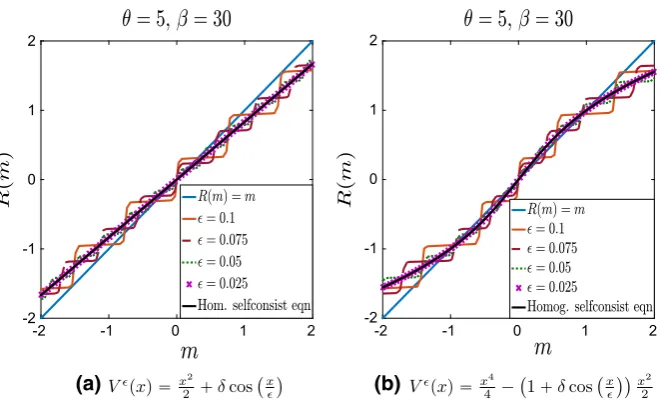
Fig. 3 Plot ofR(m;θ, β)forθ =5, β =30, δ=1 and various values offor separable potentials. aConvex potentialV0(x)andbbistable potentialV0(x). For comparison, we also plot the liney=xin
solid blue and the solution of the homogenized self-consistency equation in a solid black line (Color figure online)
Corollary 3.2 Separable fluctuations do not affect the bifurcation diagram in the mean field limit.
Proof When the fluctuations are separable (i.e., V1(x,y) does not depend on x),
ψ(x, β)in (2.24), (2.26) becomes a constant that we can ignore since it also appears in the partition function and they cancel out. Similarly, the terms of the form
Re−βV1(x,y) dy in Eqs. (3.9) and (3.10) become constants independent of x and
cancel with the corresponding terms in the partition function (3.7).
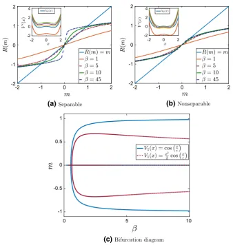
To illustrate the fact that the two limits do commute when the fluctuations are independent of the macroscale, we present in Figs.3and4the plots ofR(m;θ, β) for various values ofand fixedβ andθ, which we compare with the solution of the homogenized self-consistency equationR(m;θ, β)=m. We present results both for a convex and nonconvex confining potential, with periodic fluctuations. More details about the two-scale potentials that we use for the numerical simulations will be given in Sect.4.
As is evident from Fig.2a, the oscillatory part of the potential introduces (infinitely many) additional local minima. Consequently, Tugaut (2014), the self-consistency equationR(m;θ, β)=mhas multiple solutions. Furthermore, as shown in Fig.3b, in the limit → 0, the curves R(m;θ, β) (various dashed lines) approach those given by R(m;θ, β)computed from Eq. (2.24) (full black line), in accordance with Corollary3.2, showing the commutativity of the two limits.
[image:16.439.56.387.52.253.2]-2 -1 0 1 2
-2 -1 0 1 2 -2-2 -1 0 1 2
-1 0 1 2
(a) (b)
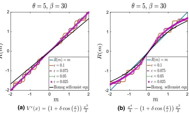
Fig. 4 Plot ofR(m;θ, β)forθ=5, β=30, δ=1 and various values offor nonseparable potentials. aConvex potentialV0(x)andbbistable potentialV0(x). For comparison, we also plot the liney=xin solid blue and the solution of the homogenized self-consistency equation in a solid black line (Color figure online)
flattened aroundx = 0. In Fig.4, we present curvesR(m;θ, β)for nonseparable fluctuations, compared with the line R(m;θ, β) = m(or y = x). We observe that in the limit→0 the curvesR(m;θ, β)(various dashed lines)do notconverge to R(m;θ, β)corresponding to the homogenized problem (full black line), in accordance with Prop.3.1. Notice also the flatness ofR(m;θ, β)aroundm=0 for smaller values of, which follows from the flatness of the corresponding potentialsVaroundx=0.
3.2 Multiscale Analysis for the McKean–Vlasov Equation in a Two-Scale Confining Potential
In this section, we study the problem of periodic homogenization for the McKean– Vlasov equation in a locally periodic confining potential, for the Curie–Weiss quadratic interaction and in one dimension. We only present formal arguments. The rigorous analysis of this problem will be presented elsewhere.
We consider the nonlinear Fokker–Planck equation (3.2) withF(x)= x22:
∂p
∂t =β
−1∂2p
∂x2 +
∂ ∂x
V0(x)p+V1
x,x
p+θ(x−m)p
, (3.11)
with initial conditions p(x,0) = pi n(x), independent of and where the prime
denotes differentiation with respect to x. The PDE (3.11) is coupled to the self-consistency equation
m(t)=
Rx p
[image:17.439.57.386.52.250.2]This homogenization problem is (slightly) different from the standard one for the Fokker–Planck equation in a two-scale potential that was studied in Duncan et al. (2016a), Duncan et al. (2016b) due to the self-consistency equation (3.12). In par-ticular, in addition to the standard two-scale expansion for the solution of the Fokker–Planck equation (3.11), we also need to expand the solution of (3.12) into a power series in:
p(x,t)= p0
x,x
,t
+p1
x,x
,t
+2 p2
x,x
,t
+. . . , (3.13a)
m =m0+m1+2m2+. . . , (3.13b)
where, as usual (Pavliotis and Stuart2008), we take{pj = pj(x,·,t) , j =0,1, . . .}
to beL-periodic in their second argument. Substituting (3.13) into (3.11) and (3.12) and using the standard tools from the theory of periodic homogenization, e.g., Fredholm’s alternative, we obtain the homogenized equation (2.19), satisfied by the marginal of the first term in the two-scale expansion p(x,t)=0L p(x,y,t)dyand with the partial free energyψ(x)given by (2.20) and with
m(t):=m0(t)=
R
L
0
x p0(x,y,t)dydx.
The convergence of m(t)tom(t)can be justified using the a priori estimates on moments of the solution to the McKean–Vlasov equation that were derived in Arnold et al. (1996), in particular (Arnold et al.1996, Eqs. (3.1), (3.2)).
Alternatively, we can work with the backward Kolmogorov equation: We recall that Eq. (3.11) corresponds to the McKean SDE
dxt = −
V(xt)+θ(xt−m)
dt+
2β−1dB
t, (3.14)
withV(x)=Vx,x. We introduce the auxiliary variableyt =xt, see, e.g.,
Pavli-otis and Stuart (2007), and using the chain rule, we can write (3.14) as a system of interacting diffusions across scales, driven by the same Brownian motion,
dxt = −
∂xV(xt,yt)+
1
∂yV(xt,yt)+θ(xt−m)
dt+
2β−1dB
t, (3.15)
dyt = −
1
∂xV(xt,yt)+
1
2∂yV(xt,yt)+
θ
(xt−m)
dt+
2β−1
2 dBt. (3.16)
reads (neglecting terms ofO()that are due to the expansion ofm)
∂u
∂t =
1
2L0+ 1
L1+L2
u, (3.17a)
u(x,y,0)= f(x,y), (3.17b)
with
L0= −∂yV∂y−β−1∂2y,
L1= −(∂xV −θ(x−m0)) ∂y−∂yV∂x−2β−1∂x∂y, L2= −(∂xV −θ(x−m0)) ∂x−θm1∂y−β−1∂x2,
We can now proceed with the analysis of (3.17a), first for the choice f(x)=x, i.e., the evolution of the first moment, and then for arbitrary observables. We obtain, thus, the homogenized backward Kolmogorov equation, from which we can read off the homogenized McKean SDE and the corresponding Fokker–Planck equation:
∂p
∂t =
∂ ∂x
β−1∂ (M(x)p)
∂x +M(x)
V0(x)+ψ(x)+θ (x−m(t))
p
+β−1∂M(x)
∂x p
, (3.18)
whereψ(x)= −β−1ln0Le−βV1(x,y)dy
andM(x)is defined in (2.10). For the sake of brevity, we will omit the details.
4 Numerical Simulations
In this section, we construct the bifurcation diagram for the stationary McKean–Vlasov equation (both for finite values ofand in the homogenization limit), present the results of Monte Carlo (MC) simulations based on the numerical solution of the particle/SDE approximation and also solve the time-dependent McKean–Vlasov PDE. Our goal is to investigate numerically the issue of (lack of) commutativity of the mean field and homogenization limits. We consider interacting diffusions (and the correspond-ing McKean–Vlasov) in one dimension and we study two types of large-scale and fluctuating parts of the potential. We consider both convex and nonconvex potentials, and both additive (separable) and multiplicative (nonseprarable) fluctuations. The four potentials that we use for our simulations are tabulated in Table1. We remark that the nonseparable fluctuations V1×(x)are truncated outside the interval[−a,a]in order to prevent the oscillations from growing as|x| → +∞.6We note that this is neces-sary for the proof of the homogenization theorem in Duncan et al. (2016b) and that,
6 In Table1, we denote byχ
Table 1 Potentials used for the numerical simulations
Confining potentialV0(x) Fluctuating potentialV1(x) Case
V0c(x)= x22 V1+(x)=δcosx 1
V1×(x)=δχ[−a,a](x)x22 cosx 2
V0b(x)=x44−x22 V1+(x)=δcosx 3
V1×(x)=δχ[−a,a](x)x22 cosx 4
furthermore, it ensures that the a priori estimates on the moments from Arnold et al. (1996) hold.7
Throughout this section, we consider fluctuations which have period L =2π. In all cases, we will consider the Curie–Weiss interaction potential F(x) = x22, and throughout Sections4.1and4.2, we will fix the interaction strength to beθ = 5. We choose this value because larger values ofθ allow for bifurcations to occur at higher temperatures, i.e., lowerβ, which is easier to handle numerically. In fact, the relevant bifurcation parameter for our problem is given by the combinationβθ; see Eq. (1.10). Fixingθ allows us to construct the bifurcation diagram by varying only the temperature. It is also clear from Eq. (1.10) that this equation has no solutions for negative values ofθ, i.e., that no (pitchfork) bifurcations can occur forθ <0.
Using Eq. (2.16), we note that the diffusion coefficient for separable fluctuations in the potential is independent ofxand is given by
M+(x)= 1
1 2π
2π 0 e−βV
+
1 (x,y)dy 1
2π
2π 0 eβV
+ 1 (x,z)d z
= 1
I0(β)I0(−β), (4.1) whereI0(·)is the modified Bessel function of the first kind (Duncan et al.2016a). On the other hand, for nonseparable fluctuations (cases 2 and 4 in Table1) we obtain
M×(x)= 1
1 2π
2π 0 e−β
V1×(x,y)dy 1 2π
2π 0 eβ
V1×(x,z)d z=
1
I0
βx2
2
I0
−βx2
2
.
(4.2) Furthermore, we obtain the following formulas for the partition functions
Z+(x)=e−β
V0(x)+θ
x2
2−mx
I0(β), Z×(x)=e−β
V0(x)+θ
x2
2−mx
I0 β x2
2
.
(4.3) We can now solve the self-consistency equation (1.9) and the equation for the critical temperature (1.10) for the various potentials given in Table1. We will track each branch of the bifurcation diagram using arclength continuation, which will enable us
7 The moment bounds in Arnold et al. (1996) were obtained for confining potentials with no oscillatory
to plot the first momentmas a function of the inverse temperatureβfor a fixed value of the interaction strengthθ. We do this using the Moore–Penrose quasi-arclength continuation algorithm.8The stability of each branch was determined in two different ways: First, we checked whether it corresponded to a local minimum or maximum of the confining potential. Second, we solved the time-dependent McKean–Vlasov equation—see details in Sect.4.5—using a perturbation of the steady state belonging to each branch (for a particular value of β andθ) as initial condition. Finally, we have confirmed the stability of each branch by computing the free energy (1.5) of a steady state from that branch at a particular value ofβ, chosen so that all the branches plotted were present. Stable branches, plotted in blue in all the figures presented in this section, correspond to local minimizers of the free energy functional; unstable branches, plotted in red, correspond to local maxima of the free energy.
4.1 Mean Field Limit of the Homogenized System of SDEs: The
→0, N → ∞Limit
As discussed before (see discussion of Corollary3.2), when the fluctuations are separa-ble the partial free energyψ(x)defined in Eq. (2.20) drops out from the homogenized stationary Fokker–Planck equation. This implies, in particular, that the invariant mea-sure(s) of the homogenized dynamics is(are) independent of the fluctuating part of the potential. In particular, there are still no phase transitions when the large-scale part of the potential is convex and still only one pitchfork bifurcation for the bistable potential case—see Fig.5—where two new, stable, branches emerge from the zero mean solution. We note that in this case the homogenized confining potential in the homogenized equation depends on the inverse temperatureβ; see the inside panels in Fig.5. In particular, the values of the local minima of the effective potential are shifted, although their location remains the same, and there are no changes in the topology of the bifurcation diagrams.
For nonseparable fluctuations, the mean field and homogenization limits do not commute (see Prop.3.1). In fact, the homogenization procedure can convexify the effective potential, and we still see no bifurcations when the large-scale part of the potential is convex, while for the bistable potential there is still only one phase tran-sition. The effect of fluctuations on the bifurcation diagram is visible by a shift of the critical temperature at which the phase transition occurs.
8 Rigorous mathematical construction of the arclength continuation methodology can be found, e.g.,
in Krauskopf (2007) and Allgower and Georg (1990). Some useful practical aspects of implementing arclength continuation are also given in Dhooge et al. (2006). We useMatlab’s toolboxes to compute the integrals in (2.24) and (2.25) and thus need to solve
F([p,m])=
p−p∞(x;θ, β,m) m−R(m;θ, β)
=0, and G(β)=β− 1
θx2p∞(x;θ, β,0)dx =0,
wherep∞(x;θ, β,m)is a stationary solution of the McKean–Vlasov equation. We start the algorithm at a sufficiently largeβ0, i.e., at a sufficiently low temperature for which we have a good initial guess for the
-2 -1 0 1 2
-2 0 2 4
-2 -1 0 1 2 -2-2 -1 0 1 2
-1 0 1 2
-2 0 2 -2-2 0 2
0 2 4
0 5 10
-1 -0.5 0 0.5 1
(a) (b)
(c)
Fig. 5 Plot ofR(m;θ, β)compared to the diagonaly=x(R(m;θ, β)=m) forθ =5, δ=1,a=5 and various values ofβfor the homogenized bistable potentials withaseparable fluctuations (potentials for various values ofβshown on the inside panel), andbnonseparable fluctuations (potentials for various values ofβshown on the inside panel).cBifurcation diagram ofmas a function ofβfor the potentials in (5a) (full line) and (5b) (dashed line)
Since there are no phase transitions for the convex potential (cases 1 and 2 in Table 1), we do not present numerical results for this case. We present in Fig. 5
[image:22.439.50.389.51.408.2]-2 -1 0 1 2
-2 0 2 -1
0 1 2 3
-2 -1 0 1 2 0 10 20 30 40 50
-1 0 1
(a) (b)
Fig. 6 Results for case 1: convexV0cwith separable fluctuations, forθ=5, δ=1, =0.1.aR(m;θ, β)
for various values ofβ, with the potentialV(x)(full line) compared withV0c(x)(dashed line) in the inside panel.bBifurcation diagram ofmas a function ofβ. Full lines correspond to stable solutions, while dashed lines represent unstable ones
4.2 Mean Field Limit of the Multiscale System of SDEs: Effects of Finite In this section, we present numerical results on the bifurcation diagram when we first pass to the mean field limit, while keepingsmall but finite. We are particularly interested in the finiteeffects on the bifurcation diagrams for the two-scale potentials presented in Table1.
4.2.1 Convex Confining Potential with Separable and Nonseparable Fluctuations
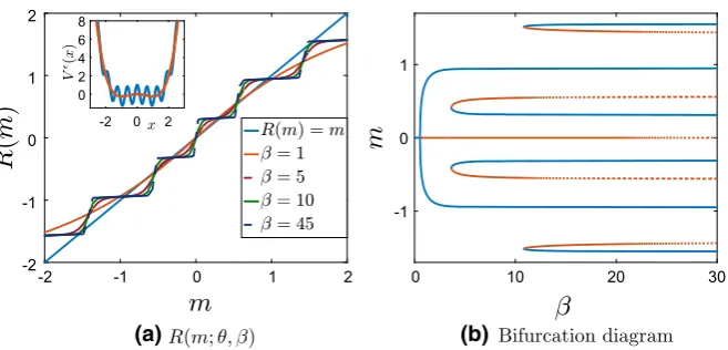
We first consider Case 1 in Table 1: a convex large-scale potential with separa-ble fluctuations. We present in Fig.6 the solution to the self-consistency equation R(m;θ, β) = m, the two-scale potential, and the bifurcation diagram for this case. For all finite values of, the resulting potential is nonconvex. This results in the self-consistency equation having multiple solutions (in fact, as→0, there are infinitely many solutions). In addition to the emerging pitchfork bifurcation (second-order, or continuous, phase transition), we observe the emergence of discontinuous branches that correspond to metastable states, since they are not (global) minimizers of the free energy; see the results presented in Table2.
Next, we consider the second case in Table1: a convex large-scale potentialV0c(x) with nonseparable fluctuations. Similarly, we present in Fig.7the solution to the self-consistency equation R(m;θ, β) =m, the two-scale potential and the bifurcation diagram. We note that, as we mentioned before, we restrict the nonseparable fluctu-ations to a finite interval. In our computfluctu-ations, we usea = 5, in the characteristic function in Table1.
[image:23.439.56.386.57.209.2]mean-Table 2 Free energy of a steady state in each branch of Figs.6,7,
8and9for fixed values ofβ
Figure 6 7 8 9
β 45 29 20 8
Free Energy 0.3080 0.1441 −0.5827 −1.7409 0.3066 0.3684 −0.5674 −0.9933
−0.4600 0.1433 −1.0918 −0.8241
−0.3908 0.3184 −0.7727 0.0856
−0.8593 0.0976 −0.8868
−0.6514 0.2425 −0.6903 0.0625
0.0630 0.0586
-2 -1 0 1 2
-2 0 2 0
2 4
-2 -1 0 1 2 0 10 20 30
-2 -1 0 1 2
β 29
F
ree Energy
0.1441 0.3684 0.1433 0.3184 0.0976 0.2425 0.0625 0.0630
0.0586 00 10 20 30 40 50
0.2 0.4 0.6 0.8
(a) (b)
(c) (d)
[image:24.439.55.391.64.504.2]zero solution remains the global minimizer of the free energy for all values ofβ. This is tabulated in Table 7c, where they are listed in the same way as in Table2, i.e., in decreasing order of nonnegative m. The free energies of the different branches are presented in Fig.7d. These new branches correspond to metastable states.
We have checked the stability of each branch by computing the free energy (1.5) of a steady state from that branch at a particular value ofβ, chosen so that all the branches plotted were present. We summarize the results in Table2. Since we only consider symmetric potentials, it is sufficient to calculate the free energy for the branches with, say, nonnegative values ofm. In each column of Table2, the values of the free energy are presented from the branch with largest value ofm to the lowest; the last value presented in each column corresponds to the branch withm=0. We summarize the results in Table2.
We observe that the branch corresponding to a pitchfork bifurcation (i.e., second-order phase transition), when present, has the lowest value of the free energy, i.e., it is the globally stable one. Furthermore, when a pitchfork bifurcation does not occur— see Fig.7—the branch corresponding tom=0 is the one with the lowest value of the free energy. Finally, we observe that the stability of the branches in Fig.9b does not alternate in the same manner as in the previous figures. This is due to the flatteness of the potential aroundx=0 for nonseparable oscillations.
The results on the stability of the different branches that are reported in this section are preliminary. A more thorough study of the local (linear) and global stability of the stationary states of the McKean–Vlasov dynamics in multiwell potentials will be presented elsewhere. We mention in passing the early rigorous work on the global stability of the steady states for the McKean–Vlasov equation in Tamura (1987) as well as the careful study of the connection between the loss of linear stability of the uniform state and phase transitions for the McKean–Vlasov equation on the torus (without a confining potential) and with finite-range interactions in Chayes and Panferov (2010).
4.2.2 Bistable Confining Potential with Separable and Nonseparable Fluctuations
Here we consider cases 3 and 4 in Table1, the bistable potentialV0b(x). In this case, the large-scale potential exhibits a second-order phase transition even in the absence of small-scale fluctuations (see the pitchfork bifurcation in Fig.1b) due to the existence of two local minima forV0b(x). We are interested in analyzing the topological changes that rapid oscillations in the potential induce to the bifurcation diagram.
We start with separable potentials—see Fig.8. We observe that the self-consistency equation R(m;θ, β)=mexhibits a larger number of solutions for finite, which, as for the convex case, result in the emergence of metastable states that are not con-tinuously connected with the mean-zero Gibbs state.
-2 -1 0 1 2
-2 0 2 0
2 4 6 8
-2 -1 0 1 2 0 10 20 30
-1 0 1
(a) (b)
Fig. 8 Results for case 3: bistableV0bwith separable fluctuations, forθ=5, δ=1, =0.1.aR(m;θ, β)
for various values ofβ, with the potentialV(x)(full line) compared withV0b(x)(dashed line) in the inside panel.bBifurcation diagram ofmas a function ofβ. Full lines correspond to stable solutions, while dashed lines represent unstable ones
-2 -1 0 1 2
-2 -1 0 1 2
-2 0 2 0
2 4 6 8
0 5 10
-1 0 1
(a)
(b)
Fig. 9 Results for case 4: bistableV0bwith nonseparable fluctuations, forθ = 5, δ = 1, = 0.1.a
R(m;θ, β)for various values ofβ, with the potentialV(x)(full line) compared withV0b(x)(dashed line) in the inside panel.bBifurcation diagram ofmas a function ofβ. Full lines correspond to stable solutions, while dashed lines represent unstable ones
4.3 Numerical Study of the Critical Temperature as a Function of
Here we study the influence of finiteon the critical temperatureβC, the solution
of (3.10) for two-scale potentials, after which continuous phase transitions (pitchfork bifurcations) occur. We do this by solving the equation (we only consider symmetric potentials)
θ−1β−1=
Rx
2
p∞(x;θ, β,m=0)dx, (4.4)
[image:26.439.57.386.53.211.2] [image:26.439.54.388.270.426.2]0 2 4 6 8 10
0.2 0.3 0.4 0.5 0.6
0.2 0.4 0.6 0.8 1 0.2 0.4 0.6 0.8 1 0.30 0.05 0.1 0.15 0.2
0.4 0.5 0.6 0.7
[image:27.439.53.385.54.161.2](a) (b) (c)
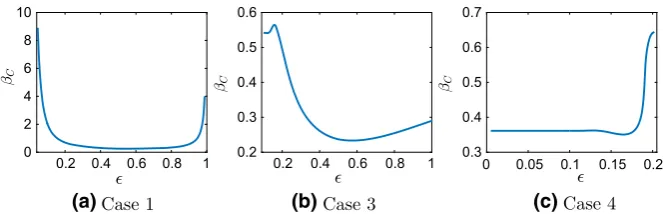
Fig. 10 Critical temperatureβCas a function offor the multiscale Fokker–Planck equation withθ=5 for casesa1−V(x)= x22 +δcosx,b3−V(x) = x44 − x22 +δcosx, andc4−V(x) =
x4
4 −
x2
2
1−δcosxin Table1
We present in Fig.10plots of the critical temperature,βC as a function offor
a fixedθ = 5. The results are presented for cases 1 (Fig.10a), 3 (Fig.10b) and 4 (Fig.10c) from Table1. We do not present the remaining case because, as shown in Fig.7b, there is no pitchfork bifurcation from the mean-zero solution for case 2. The dependence of the critical temperature onis different for separable and nonseparable potentials. It appears that the critical temperature can change considerable by varying
, which implies that a different number of branches might be present in the bifurcation diagram at a fixed temperature, for different values of. This issue will be studied in detail in future work.
4.4 Simulations of the Interacting Particles System
In this section, we present the results of Monte Carlo (MC) simulations for the system of interacting diffusions, both for the full, i.e.,-dependent, (2.1) and for the homogenized dynamics (2.17). Our focus is on the study of the convergence of the interacting particles system to their equilibrium state. It should be emphasized that no phase transitions occur for the finite-dimensional particles system. However, the numerical simulation of the two interacting particles systems, (2.1) and the homogenized particle system (2.17) clearly exhibit the lack of commutativity between the mean field and homogenization limits.
For the full dynamics (2.1), we usedδ=1 and=0.1. We solved the SDEs using the Euler–Maruyama scheme. For the homogenized dynamics (2.17), since the noise is multiplicative (for nonseparable potentials), we used the Milstein scheme. In both cases, the time step used was dt =0.01, which is ofO(2). Finally, in both cases we initialized theNparticles as being normally distributed, with mean zero and variance 4, which was large enough so that all the local minima were contained within two standard deviations of the Gaussian distribution.
-5 0 5
200 400 600 800 1000 -5 200 400 600 800 1000
0 5
-5 0 5
200 400 600 800 1000 -5 200 400 600 800 1000
0 5
-5 0 5
200 400 600 800 1000 -5 200 400 600 800 1000
[image:28.439.51.387.53.482.2]0 5
Fig. 11 Position ofN =1000 particles forV(x)= x22 +δcosx, withθ =2,β=8,δ=1. Left: Eq. (2.1) with=0.1. Right: homogenized SDEs (2.17)
the results for=0.1, while the right panels show the results for the homogenized system. In Fig.12, we present snapshots of the histogram for theN =1000 particles for the same time and parameter values, which are δ = 1, = 0.1, θ = 2 and
Fig. 12 Histogram ofN=1000 particles forV(x)= x22 +δcosx, withθ=2,β=8,δ=1. Left: Eq. (2.1) with=0.1. Right: homogenized SDEs (2.17)
We also calculate the empirical average of the interacting particle system
¯ XtN := 1
N
N
i=1
Xit, (4.5)