Optimum Multi DG units Placement and Sizing
Based on Voltage Stability Index and PSO
J. J. Jamian1, M.M. Aman2[email protected], [email protected]
M.W. Mustafa1, G.B. Jasmon2 [email protected], [email protected]
H. Mokhlis2, A.H.A. Bakar2 [email protected], [email protected]
M.N. Abdullah3 [email protected]
1Faculty of Electrical Engineering, Universiti Teknologi Malaysia, 81310 UTM Johor Bahru, Malaysia. 2Faculty of Engineering, University of Malaya, 50603 Kuala Lumpur, Malaysia.
1Faculty of Electrical Engineering, Universiti Tun Hussien Onn, 86400 Johor Bahru, Malaysia.
Abstract-Optimum DG placement and sizing is one of the current topics in restructured power system. Most of the authors have worked out on their optimum placement base on the power losses reduction concept. However, the improvement on power losses value in the network will not guarantee to the planner to have lower voltage stability index (VSI) for the system. This paper proposes a new approached for multi DG placement and sizing for distribution systems which is based on a voltage stability index. The most optimum DG size will be found out using several types of PSO optimization algorithm. The output results will also compared with EPSO, REPSO, and IPSO. The proposed algorithm is tested on 12-bus, modified 12-bus and 69-bus radial distribution networks.
Index Terms—Multi-DG placement, PSO, Voltage Stability Index, DG sizing
I. INTRODUCTION
Distributed Generation placement and sizing is one of the major issues of power system, particularly after restructuring of power system. Many companies are investing in small scale power generation. In England and Wales, DG production was only 1.2 GW during 1993-1994. However today this figure has increased substantially and reached up to over 12 GW [1]. According to Energy Network Association (ENA) report [2], the UK government is targeting to achieve 15% of electricity from the renewable sources by 2015.
However there are several issues concerning the integration of DGs with existing power system networks that needs to be addressed. The integration of DG changes the system from passive to active networks, which affects the reliability and safe operation of a power system network [3]. Furthermore, the non-optimal placement and sizing of DG can result in an increased system losses and thus making the voltage profile lower than the allowable voltage limit [3-5].
The increment in active power loss represents loss in savings to the utility as well as a reduction in feeder utilization. Studies have shown that 70% of power losses are due to distribution system [6] and the losses resulting from Joule effect only account for 13% of the generated energy [7] . This non-negligible amount of losses has a direct impact on the financial results and the overall efficiency of the system. The unbundling of utility has forced the distribution
companies to reduce the losses and operate at the highest efficiency for their own economical benefits. Since utilities are already facing technical and non-technical issues, they cannot tolerate such additional issues. Hence an optimum placement of DG is needed in order to minimize overall system losses and therefore improve voltage profiles.
Different approaches have been used to get the optimal placement of DG such as using the maximum power losses reduction indicator [8], heuristic optimization technique [9-10] and others. However, in this study, the allocation of the DG will be based on the weak node or bus that can cause the system near to collapse point and the DG will be placed on the weakest bus. Voltage stability index will be developed to identify the weakest bus and the optimization algorithm will be applied to find the most optimum DG size. The proposed algorithm will be tested on 12-bus and 69-bus radial distribution networks.
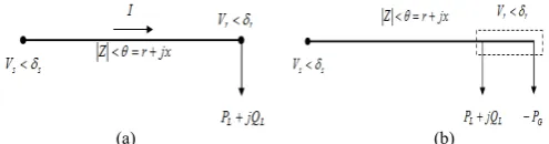
II. DEVELOPMENT OF VOLTAGE STABILITY INDEX To identify the weakest bus in the system, the voltage stability index is developed to give the indication for the stability of the buses and also the effect of DG will be incorporated. For derivation of the index, a simple two bus network is considered, shown in Fig. 1.
[image:1.595.307.555.526.591.2](a) (b) Fig. 1: A Simple Two Bus Network with and without Active Power
Compensation From Fig. 1, we can write.
* r r L L
L P jQ V I
S = + = (1) Z
I V
Vr = s− r (2) Where,
*
) (
) (
r
G L G L r
V
Q Q j P P
Solving Eqns. (1-3), the following relation could be derived.
[
( )]
1) ( 4 2 ≤ − −
δ
θ
Cos V P P r i G L ij (4)This new index is based on active power value (due to the DG that operating in PQ mode) is derived for finding the most optimum site of DG based on the most critical bus in the system that can lead to system instability. This proposed index is referred as real power system stability index (PSI) as defined in (5).
[
( )]
1) ( 4 2 ≤ − − =
δ
θ
Cos V P P r PSI i G L ij (5)Under the stable operation, the PSI should be less than unity and if the PSI value is closer to zero, the system at stable condition.
III. OPTIMIZATION TECHNIQUES IN DGSIZING
The optimization technique will be implemented in DG sizing to obtain its optimal value after the allocation of DG has done. By having the optimal size of DG, it will help the system to have the minimum power losses compared to the initial condition. Many optimization techniques have been employed to solve different DG units’ problems. This includes Artificial Bee Colony (ABC), Genetic Algorithm (GA), Simulated Annealing (SA), Evolutionary Programming (EP) and Particle Swarm Optimization (PSO). [11-13]. Some of these techniques also have been modified to enhance their performance to overcome other limitations [14-15]. However, the PSO algorithm has more advantages as compare to others optimization methods. PSO algorithm is easier to be implemented, less memory required, has ability to reach global optimum solution and also can obtained good solution in a short computing time [16].
Four different types of PSO are used in this study to obtain the optimal DG size. This includes Traditional PSO, Evolutionary PSO (EPSO), Rank Evolutionary PSO (REPSO) and Iteration PSO (IPSO). The second and third PSO types are the hybridization of PSO with the Evolutionary Programming technique while the last PSO types is the modification on PSO algorithm that in introduce by [17]. The objective function for all the optimization techniques is to determine the minimum total active power losses as shown in Eqn. (6): ⎪⎭ ⎪ ⎬ ⎫ ⎪⎩ ⎪ ⎨ ⎧ =
∑
= n i i iLt I R
P Min 1 2 (6)
A. Traditional Particle Swarm Optimization
The traditional Particle Swarm Optimization (PSO) is implemented from the behavior of population such as fish, birds and others animal to find their food source. This
population will remain moving in the group based on the experience or information that is achieved by individual or group. This idea is used in the PSO algorithm [18].
From the random number (particles) that is generated by the computer. The Local Best (Pbest) and Global Best (Gbest)
parameters are introduced to help these random particles to move toward the optimal solution (highest density of food source). The Pbest is defined as the best result (minimum or
maximum) that is achieved by individual particle until the current iteration and Gbest is the best result that is obtained
from the whole population. Besides that, there are 3 weight coefficients in the PSO algorithm which are w, c1 and c2. All
weighted coefficients will affect the performance of PSO in exploring or exploiting the global results. Eqn. (7) and (8) show the updated velocity and position of the particles until obtaining the optimal solution.
) (
)
( 2 2
1 1
1 i best i best i
i V cr P x c r G x
v+ =ω + − + − (7)
i i
i v x
x+1= +1+ (8)
B. Evolutionary Particle Swarm Optimization
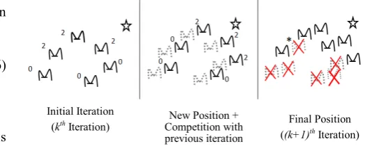
The Evolutionary Particle Swarm Optimization (EPSO) is an improvement method that is introduced by [19] for avoiding trapping in local optimal value and make the algorithm to have faster computing time. The concept of Evolutionary Programming (EP) is hybridized inside the PSO algorithm for improving its performance. Since the EP consist of combination, competition and selection process, it make only the winning (high potential) particle will remain in the group while the others will be terminated. Fig. 2 illustrated the way of competition that is done for PSO particles. The “star” is presented as the optimal solution that needs to be achieved by the algorithm. The previous population is combined with the current population (updated ones) and the competition is based on the percentage that is set by the user. Let the number of particles (N) are 6 and the competition rate are 25%, each particles will randomly competed with others 2 particles. When the particles have better results (minimum or maximum based on objective function) compared to its competitor, the particles will obtained 1 point. The process is repeated until all particles have done the competition. Finally, only the highest winning point will remain as survival particle for next iteration.
Initial Iteration
(kth Iteration) Competition with New Position +
previous iteration
[image:2.595.287.549.596.701.2]Final Position ((k+1)thIteration)
C. Rank Evolutionary Particle Swarm Optimization
The Rank Evolutionary Particle Swarm Optimization (REPSO) is an improvement technique for the EPSO methods. The competition concept that is used in EPSO analysis might cause the “lucky” particle still surviving in the next iteration. From the Fig. 2, the *-particle is deleted due to the lower mark even though it has better fitness value compared to other survival particles. Thus, in the REPSO, the competition concept is replaced with the ranking concept. After the combination between previous and current iteration, all particles will be rank based on its fitness value and the top N from the total population will be selected as survival particle while the others will be deleted. This process will make the only best result remained in the population and achieved the optimal solution in shorter time. The others process of REPSO is same as in EPSO algorithm.
[image:3.595.305.551.393.715.2]Table 1 shows the example of REPSO process in determining the survival particles. Let all the values in the table as the fitness value of each particle in Fig. 2 and the objective function is to find maximum value of a function. Column 2 presents the previous fitness values that are achieved by the particles and the column 3 presents the current iteration fitness values. After the ranking process (column 4), only 6 number of particles remained for the next iteration and the others are deleted. Therefore, the ranking process will sort the potential particles at the top ranking for them to survive in the next iteration.
Table 1: The example of REPSO algorithm process in finding the maximum fitness function
Particle k-th
iteration iteration k+1-th Combination Ranking Selection
No. 1 6.845 6.458 6.845 7.421 7.421
No. 2 7.214 7.421 7.214 7.214 7.214
No. 3 3.125 3.013 3.125 6.845 6.845
No. 4 6.127 6.478 6.127 6.478 6.478
No. 5 4.025 4.125 4.025 6.458 6.458
No. 6 6.389 6.446 6.389 6.446 6.446
6.458 6.389
7.421 6.127
3.013 4.125
6.478 4.025
4.125 3.125
6.446 3.013
D. Iteration Particle Swarm Optimization
The Iterative Particle Swarm Optimization (IPSO) is an improvement method on solution quality and computing time which is proposed by [20]. Compared to traditional PSO, the IPSO consists of 3 best values which are Gbest, Pbest and Ibest.
The Ibest is defined as any Pbest value that is selected randomly
among existing particles in that present iteration. After the selection process, the current Ibest value will be compared with
previous Ibest. If the current Ibest is better than previous result,
the value of Ibest will be remained and be used to update the
position of the particles. Otherwise, the previous iteration Ibest
will be used in the calculation. The process of Pbest and Gbest
in the IPSO is same as traditional PSO. Furthermore, the different approached on acceleration coefficient for the Ibest is
used where the authors used dynamic acceleration techniques rather than a constant value. This c3 value will change base on
c1 parameter value and the number of iteration as stated in
(9).
)
1
.(
.1
3
c
e
c1kc
=
−
− (9) Where:k = number of iteration
Therefore, the new velocity formula for the IPSO algorithm will have additional coefficients compared traditional PSO as shown in (10).
) x I )( e .( c
) x G ( r c ) x P
( r c v v
k i k best k . c
k i k best k
i k
i best k
i k k i
− −
+
− +
− +
=
− − +
1 1
1
2 2 1
1 1 ω
(9)
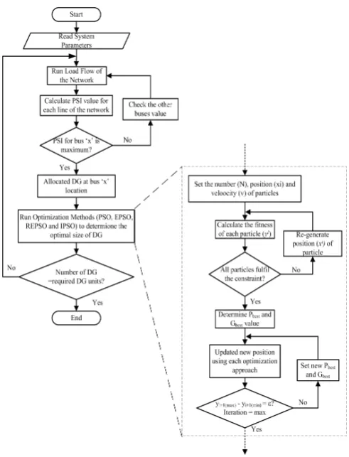
[image:3.595.42.300.416.592.2]IV. PROPOSED ALGORITHM FOR OPTIMAL ALLOCATION AND SIZING OF DGUSING PSI AND VARIES PSOMETHODS Fig. 3 shows the process to allocate and size either a single or multiple DG units in the distribution network using PSI and varies PSO technique.
The left side of the figure is explaining the process to allocate the DG using PSI technique and the “zoom in” part of the figure shows the procedure to determine the optimal DG size using optimization technique. After the allocation of the DG has done with the optimization results, the whole system is assumed as the base case for the 2nd allocation of the DG and continues until specific number of DG has allocated. However, in this study, only two DG units will be allocated for 12 bus and 69 bus test systems.
V. SIMULATION AND RESULTS A. Test System
[image:4.595.323.537.53.210.2]The proposed algorithm is tested using 12-Bus [21] and 69-Bus [22] radial distribution networks shown in Figs. 4 and 5.
[image:4.595.47.287.254.457.2]Fig. 4. Single Line Diagram of 8-Bus Radial Network
Fig. 5. Single Line Diagram of 69-Bus Radial Network
B. Calculation of PSI
[image:4.595.335.520.324.470.2]The PSI values for each line are found out using Eqn. (5). The calculated values for each line of each case are shown in Figs. 6 and 7.
Fig. 6. Single Line Diagram of 69-Bus Radial Network
Fig. 7. Single Line Diagram of 69 Bus Radial Network
From Figs. 6 and 7, it could be visualized that the DG should be placed at the end of line 8 (9th bus) and line 60 (61th bus) in 12-bus and 69-bus test systems respectively.
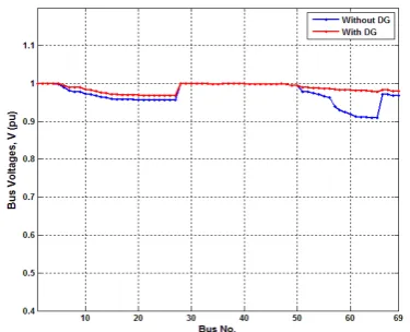
C. System Voltage Profile
[image:4.595.333.521.504.656.2]In order to show the improvement in voltage buses, voltage profile for 12-bus and 69-bus distribution network is plotted in Figs 8 and 9, respectively.
Fig. 8. Effect of DG on System Voltage Profile of 12-Bus system
Fig. 9. Effect of DG on System Voltage Profile of 69-Bus system
[image:4.595.67.269.555.693.2]D. Sizing of DG (Optimization Techniques)
Once the optimum DG location is found out, optimum DG size is calculated using PSO, EPSO, REPSO and IPSO algorithms. The computed results are shown in Table I-IV.
The optimum DG size and the effect on power losses are shown in Table I and III. However performances of optimization theorems are given in Table II and IV.
1st DG Placement:
TABLE I
DGSIZING AND LOSSES AFTER ALLOCATION OF 1STDG PLACEMENT
No Test Systems Location DG DG Size (MW) Power Losses (KW)
PSO EPSO REPSO IPSO PSO EPSO REPSO IPSO
1 69-Bus 61 1.87270 1.87265 1.87256 1.87270 0.08322 0.08322 0.08322 0.08322
2 12-Bus 9 0.23545 0.23542 0.23634 0.23545 0.01076 0.01076 0.01076 0.01076
TABLE II
NO. OF ITERATIONS AND COMPUTATION TIME IN 1STDG PLACEMENT
No Test Systems No of Iteration Computation Time (s)
PSO EPSO REPSO IPSO PSO EPSO REPSO IPSO
1 69-Bus 121 57 48 172 213.681360 69.003861 57.945735 181.071722
2 12- Bus 123 44 36 137 240.743952 40.630089 29.812881 105.771047
2nd DG Placement:
TABLE III
DGSIZING AND LOSSES AFTER ALLOCATION OF 2NDDG PLACEMENT
No Systems Test Location DG DG Size (MW) Power Losses(KW)
PSO EPSO REPSO IPSO PSO EPSO REPSO IPSO
1 69- Bus 64 0.04511 0.04512 0.04508 0.04511 0.08314 0.08314 0.08314 0.08314
2 12-Bus 8 0.04243 0.04259 0.04160 0.04243 0.01055 0.01055 0.01056 0.01055
TABLE VI
NO. OF ITERATIONS AND COMPUTATION TIME IN 2NDDG PLACEMENT
No Test Systems location DG No of Iteration Computation Time
PSO EPSO REPSO IPSO PSO EPSO REPSO IPSO
1 69-Bus 64 99 40 35 148 125.391516 39.110 32.418 110.810
2 12-Bus 8 119 46 35 141 158.174861 33.667 24.367 84.589
E. Discussion:
From Tables I-IV, it can be said that all PSO methods will give similar results in DG sizing and the power losses value up to the 4th decimal places. However, the number of iteration and the computing between them are different. Thus, the new PSI value for the system will be observed after the optimal DG value is obtained before the 2nd DG placement is doing. The results show that the 2nd placement of DG will give lower power losses to the network with better VSI value for the whole system. It can be conclude that, the allocation of DG base on PSI value will give positive impact on power losses reduction as well as VSI value of the system.
VI. CONCLUSION
REFERENCES
[1] Jenkins N, Ekanayake J, Strbac G. Distributed Generation - IET Factfiles Available at: www.theiet.org/factfiles/energy/distributed-generation.cfm. 2010.
[2] Energy Networks Association (UK). Available at:
http://2010.energynetworks.org/distributed-generation [accessed on 10-08-2011].
[3] Hadjsaid N, Canard JF, Dumas F. Dispersed generation impact on distribution networks. IEEE Comput Appl Pow. 1999;12:22-8.
[4] Tuitemwong K, Premrudeepreechacharn S. Expert system for protection coordination of distribution system with distributed generators. International Journal of Electrical Power & Energy Systems. 2011;33:466-71.
[5] J.J. Jamian, H. Musa, M.W. Mustaf, H. Mokhlis, S.S. Adamu, “Combined Voltage Stability Index for Charging Station Effect on Distribution Network”, International Review of Electrical Engineering-IREE, vol. 6, no. 7, December 2011, pp. 3175-3184.
[6] Lund T. Analysis of distribution systems with a high penetration of distributed generation: Technical University of Denmark; 2007.
[7] Khodr HM, Olsina FG, Jesus PMDO-D, Yusta JM. Maximum savings approach for location and sizing of capacitors in distribution systems. Electric Power Systems Research. 2008;78:1192-203.
[8] S. M. Moghaddas-Tafreshi, Elahe Mashhour, “Distributed generation modeling for power flow studies and a three-phase unbalanced power flow solution for radial distribution systems considering distributed generation”, Electric Power Systems Research, Volume 79, Issue 4, April 2009, Pages 680-686.
[9] A. Soroudi and M. Ehsan, “Efficient immune-GA method for DNOs in sizing and placement of distributed generation units”, European Transactions on Electrical Power, vol. 21, no. 3, April 2011, pp. 1361-1375.
[10] S. Ghosh, S. P. Ghoshal, and S. Ghosh, “Optimal sizing and placement of distributed generation in a network system”, International Journal of Electrical Power & Energy Systems, vol. 32, no. 8, Oct 2010, pp. 849-856.
[11] Ghosh S, Ghoshal SP, Ghosh Sa. Optimal sizing and placement of distributed generation in a network system. Int J Elec Power. 2010;32(8):849-56.
[12] M.F.Kotb, K.M.Sheb, M. El Khazenda, A. El Hussein, “Genetic Algorithm for Optimum Siting and Sizing of Distributed Generation”,
The 10th MEPCON International Middle East Power Systems Conference, December 19-21, 2010.
[13] F. S. Abu-Mouti and M. E. El-Hawary, "Optimal Distributed Generation Allocation and Sizing in Distribution Systems via Artificial Bee Colony Algorithm," Ieee Transactions on Power Delivery, vol. 26, no. 4, pp. 2090-2101, Oct.2011.
[14] G. Isazadeh, R. A. Hooshmand, and A. Khodabakhshian, "Modeling and optimization of an adaptive dynamic load shedding using the ANFIS-PSO algorithm," Simulation-Transactions of the Society for Modeling and Simulation International, vol. 88, no. 2, pp. 181-196, Feb.2012.
[15] J.J. Jamian, M.W. Mustafa, H. Mokhlis, J. Usman, “Distributed Generator Sizing: An Iteration Particle Swarm Optimization Approach”, Proceedings of the IASTED International Conference Power and Energy Systems, AsiaPES 2012, April 2 - 4, 2012, 439-444.
[16] D. Niu, Z. Gu, M. Xing,“Research on Neural Network Based on Culture Particle Swarm Optimization and its Application in Power Load Forescasting”, Third International Conference on Natural Computation. 2007.
[17] T. Y. Lee and C. L. Chen, Unit commitment with probabilistic reserve: An IPSO , Energy Conversion and Management, vol. 51, no. 12, Dec.2010, pp. 2394-2401.
[18] J. Kennedy, R. C. Eberhart,“Particle Swarm Optimization”, IEEE International Conference on Neural Networks IV, Piscataway, NJ, Vol.4, 1995 , pp. 1942—1948.
[19] Angeline, P.J., Using selection to improve particle swarm optimization, Evolutionary Computation Proceedings, 1998. IEEE World Congress on Computational Intelligence., The 1998 IEEE International Conference on , 4-9, May 1998, vol., no., pp.84-89.
[20] T. Y. Lee and C. L. Chen, Unit commitment with probabilistic reserve: An IPSO , Energy Conversion and Management, vol. 51, no. 12, Dec.2010, pp. 2394-2401.
[21] Das D, Nagi HS, Kothari DP. Novel method for solving radial distribution networks. In: IEE Proceedings-Generation, Transmission and Distribution. 1994; 141(4); 291-8.