Face Recognition Using SIFT

(1)

International Journal of Emerging Technology and Advanced Engineering

Website: www.ijetae.com (ISSN 2250-2459,ISO 9001:2008 Certified Journal, Volume 4, Issue 5, May 2014)

358

Face Recognition Using SIFT

Trasha Gupta

1

, Lokesh Garg

2

1_{Department of Computer Science, Deen Dayal Upadhyaya College,University Of Delhi, Delhi, India}

2_{Indraprastha Institute of Information Technology, Delhi, India}

Abstract— From 1970, research on automated face recognition has been on the rise. Since then many techniques and algorithms have been designed each one trying to provide better efficiency than the earlier one. This field of biometric analysis has found its use in many practical applications and with rising technologies each day, its exhaustive use in future is also expected. In this paper we have studied the efficiency of Scale-invariant feature transform (SIFT), a feature based algorithm for face recognition. This paper includes overview of the SIFT algorithm, the experiment conducted to carry out the research finding accuracy and efficiency of the algorithm. Using the experimental data and applying descriptive and inferential statistics on the obtained data, we came up with strong results that gives explored analysis of SIFT algorithm and its accuracy.

Keywords—Scale Invariant Feature Transform (SIFT), SURF.

I. INTRODUCTION

While research on the ways of making face recognition automatic exists from 1970‟s but it has received importance in the past several years only. According to the experts of the field reason behind these are wide range of commercial and law enforcement applications, security access control application and availability of feasible technologies after 30 years of research. Thousands of research papers have been written on face recognition and large number of algorithms and techniques have been proposed. Largely these methods can be divided in 2 categories namely holistic and feature based.

In holistic methods whole face was used as an input to the algorithm and then matching was done. It provided good efficiency. Its advantage over feature based recognition methods is that it considers the whole face as one feature, so there is no problem in dividing the face into features. But these were not robust to pose and expression changes. Many research papers [2-4] have been published using this method. Principal component analysis (PCA) [5] is a typical face-based technique.

In feature based methods recognition is done by selecting some local facial features like eye(s), mouth, nose and face boundary from the whole face and these local features are used as face descriptors to identify the faces uniquely.

Decision whether image is the same or impostor is done based on relationship between these features and descriptors. The difficulty in use of local features is that it become tough to efficiently find those features which are most stable and discriminative for face recognition. Deformable template is a common method used in detecting facial features. In the past decade feature based image recognition techniques have become very popular with thousands of papers written using them. Some of the famous local feature algorithms include LBP(Local Binary Pattern) [6] in which the face image is divided into several regions from which the LBP feature distributions are extracted and concatenated into an enhanced feature vector to be used as a face descriptor. SURF [1] and SIFT [7] are other most widely used feature algorithms. SURF has been showed to be robust to illuminations and SIFT works well for poses and expression invariants. This was the motivation for us to choose a feature based algorithm and analyse it‟s accuracies under different invariants like camera resolution, expressions, ambiance, accessories .So we chose SIFT because of its successful application in various general object recognition tasks.

(2)

International Journal of Emerging Technology and Advanced Engineering

359

In this paper we have worked on finding the accuracy of SIFT by first collecting the whole data from scratch and then creating a database from those images for image comparisons. Specifications for data collection and experiment procedure have been mentioned in the Experiment section. We have used various invariants (described precisely in convention section) in testing SIFT. We also observed the variation in the percentage of matching when two different images of a subject (i.e. an individual) with different features are compared with a standard base 2 image of same subject. These have been mentioned in the analysis part.

II. SIFT

In this section we give the summary of the algorithm provided in [7], [9]. For a detailed explanation please see [7]. SIFT algorithm has been divided in 4 procedures of computation.

i. Scale-space extrema detection: To detect blob structures in an image, a scale space is constructed where the interest points, which are called key points in the SIFT framework are detected. The scale space function is produced from the convolution of a

variable-scale Gaussian, G(x, y, σ2) with an input

image, I(x, y):

As studied by Lindeberg, the normalization of the

Laplacian, σ2 2_{G with the factor σ}2

is required for true scale invariance. Thus automatic scale selection is done in the image after convolution with the normalized Laplacian function:

As proved in if the scale of the image structure is close to the value of normalized Laplacian function,

the output O(x, y, σ2_{) calculated from convolution of}

the image with σ2 2

G will be extremum. Thus, to detect blob structures and represent them at the most optimal scale, the points which are extrema in both spatial and scale spaces are selected.

ii. Unreliable key point’s removal: In this step the value

of |O(x, y, σ2_{)| at each candidate key point is}

evaluated. If this value is below some threshold which means that the structure has low contrast (and is therefore sensitive to noise), the key point will be removed.

For poorly denned peaks in the scale-normalized Laplacian of Gaussian operators, the ratio of principal curvatures of each candidate key point is evaluated. If the ratio is below some threshold, the key point is kept.

iii. Orientation assignment: In this step, each key point is assigned one or more orientations based on local image gradient directions.

iv. Key point descriptor: The image gradient magnitudes and orientations are sampled around the key point location, using the scale of the key point to select the level of Gaussian blur for the image. The feature descriptor is computed as a set of orientation histograms on 16 × 16 pixel neighbourhoods around the key point. Each histogram contains 8 bins, and each descriptor contains a 4 × 4 array of histograms around the key point. Therefore, the feature vector for each key point is 4 × 4 × 8 = 128 dimension.

III. EXPERIMENT

A. Data collection protocol

Since this paper was a part of the course project we had 2 weeks for data collection and we collected images of 44 subjects using a mobile phone. We used the following constructs for our data collection:

 Ambiance: Indoor/Outdoor

 Camera resolution: 3 MP/ 2 MP

 Expression: normal/smile

 Accessories: goggles in outdoor only

Using the above constructs 14 images (8 outdoor and 6 indoor) for each subjects were captured but the images that were used for the computation are described below with convention that will be followed later.

B. Conventions and Experiment conducting Protocol

(3)

International Journal of Emerging Technology and Advanced Engineering

360

Table 1

CONVENTION TABLE FOR TEST SET

Symbol used for images

Image Name Ambiance Camera

Resolution

Expression accessories

img_A X_11_indoor_smile_3 Indoor 3MP smile No

Img_B x_1_outdoor_normal1_3 Outdoor 3MP normal No

Img_C x_3_outdoor_smile_3 Outdoor 3MP smile No

Img_D x_9_indoor_normal1_3 indoor 3MP Normal No

Table 2

CONVENTION TABLE FOR DATA SET

Symbol used for images

Image Name Ambiance Camera

Resolution

Expression accessories

img_E X_10_indoor_ normal2_3 indoor 3MP smile No

Img_F x_2_outdoor_normal2_3 outdoor 3MP normal No

Img_G x_4_outdoor_normal_goggle_3 outdoor 3MP normal goggle

Img_H x_5_outdoor_normal1_2 outdoor 2MP Normal No

Table I describes the images of “Test set”. “Data set” contain 176 images of database other than those in “Test set”. Table II describes the images of “Data set” In both the tables “x” signifies the subject number and it range from 1 to 44. Using MATLAB each image in ”test set” was made to run on SIFT algorithm which compared them to all the images in the ”Data set” and computed the number of feature matched between the two images. We calculated the percentage match between two images as

IV. ANALYSIS

As mentioned in the Experiment section that each “test set” image is compared with all the images in the database set and corresponding percentage match was calculated. For the analysis of data obtained, following two methods of getting the accuracy of algorithm were adopted.

Method 1: Computed the top 4 images with maximum matching percentage for each “test set” image.

Method 2: Computed the top 6 images with maximum matching percentage for each “test set” image.

According to top 4 and top 6 images matched for one “test set”, weights were assigned using if else classifier shown below

A. Overall Accuracy analysis

For calculating the accuracy, weights of all test cases were taken and added. This total was divided by maximum possible weight (i.e. 176 for 176 images). Percentage was calculated using the above calculations as:

This percentage was calculated for both Methods and shown as follows:

Method 1:

The total weight of the 176 subjects = 68.50

So the accuracy percentage came out to be = 38.92%

Method 2:

The total weight of the 176 subjects = 78.50

So the accuracy percentage came out to be = 44.89%

Table 3

SIFT COMPARATIVE STUDY

Name of image being compared

Points matched

%

Img_E 2 4.54

Img_F 40 90.9

Img_G 22 50

Img_H 38 86.36

Img_C 36 81.81

B. Comparative analysis

In this section we analyze how much robust SIFT is to different invariants. So to check this robustness we compared img_B with img_E, img_F, img_G, img_H, img_C separately for each subject. Procedure followed is as follows:

(4)

International Journal of Emerging Technology and Advanced Engineering

361

Else 0

Similarly same procedure for img_F, img_G, img_H and img_C is followed. Table III shows the obtained values and percentage of their comparison with img_B .

C. Statistical Comparative analysis

In this section we analyzed the comparison done in the ection 4.2 statistically. McNemar‟s test had been used in the following three cases:

Case 1: img_C v/s img_G

Hypothesis: Accuracy of matching img_C and img_G that come in top 4 with comparison to img_B is statistically same.

N00: Both were not there in top 4.

N01: Img_C was not there in top 4 and img_G was there in top 4.

N10: Img_C was there in top 4 and img_G was not there in top 4.

N11: Both were there in top 4.

If

χ

2 > 3.814 then we reject the hypothesis with 95%

[image:4.612.56.282.474.555.2]

confidence interval else the matching accuracy for both is statistically equal. The values obtained are mentioned in the table.

Table 4 McNEMAR TEST 1

McNemar

Img_G not in top 4

Img_G in top4

Img_C not in top 4 6 2

Img_C in top 4 16 20

According to the calculation from Table IV we calculate

the

χ

2

. The

χ

2 came out to be = 9.3. Since

χ

2 > 3.814 we

reject our hypothesis and conclude that these two variants are statistically not same (i.e. SIFT does not match img_B with img_G as accurately as it does for img_C).

Case 2. Img_E v/s img_G

Hypothesis: Accuracy of matching img_E and img_G that come in top 4 with comparison to img_B is statistically same.

N01: img_E was not there in top 4 and img_G was there in top 4.

N10: img_E was there in top 4 and img_G was not there in top 4.

N11: Both were there in top 4.

[image:4.612.335.556.581.643.2]

The values we got are mentioned in the table below.

McNemar Img_G not in

top 4

Img_G in top4

Img_E not in top 4 20 22

Img_E in top 4 2 0

According to the calculation from Table V we calculate the

χ

2

.The

χ

2 came out to be = 15. Since

χ

2 > 3.814 we

reject our hypothesis and conclude that these two variants are statistically not same (i.e. SIFT does not match img_B with img_E as accurately as it does for img_G).

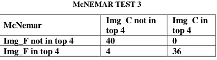
Case 3. img_F vs img_C

Hypothesis: Accuracy of matching img_F and img_C that come in top 4 with comparison to img_B is statistically same.

N01: img_F was not there in top 4 and img_C was there in top 4.

N10: img_F was there in top 4 and img_C was not there in top 4.

N11: Both were there in top 4. The values we got are mentioned in the table.

According to the calculation from Table VI we calculate

the χ2. The χ2 came out to be = 2.5. Since χ2 < 3.814, we

fail to reject our hypothesis and conclude that these two variants are statistically same (i.e. SIFT matches img_B with img_F approximately as accurately as it does for img_C).

McNemar Img_C not in

top 4

Img_C in top 4

Img_F not in top 4 40 0

(5)

International Journal of Emerging Technology and Advanced Engineering

362

V. RESULTS

After analysing all the computation on the data, we can clearly make few strong inferences about SIFT and its implementation.

 According to our database with 14 images of each

subject, SIFT came out to be 38.92% accurate when top 4 images were chosen and 44.89% when top 6 were taken. It signifies that for any random image if there is any other image corresponding to given random image then the returned image as matched image is approximately 38.92% correct or 44.89% as per method chosen.

 SIFT is not a good tool to check similarity of images

with different illumination. This can be inferred from observing Table III as accuracy of matching an outdoor image to an indoor image came out to be only 4.25%. Statistical analyses using McNemar test also supported the above result.

 When matching the image to an image with some

accessory, the accuracy came out to 50% and McNemar also proved that its accuracy is not statistically same to the accuracy of images with different expressions and camera resolution. As McNemar showed images that belong to category img_G and img_C were having statistically different accuracy and camera resolution percentage match was more than that of smile hence it would also be statistically different.

 Comparing images belonging to category img_C with

an image belonging to category img_B yielded 81% accuracy and was also showed to be statistically same by McNemar test.

 Using a different Camera resolution gave a accuracy

of 88%. This means that SIFT is capable of matching images with different camera resolutions.

VI. CONCLUSION

In this paper SIFT was used for face recognition on

different invariants and accuracy was calculated.

Comparative analysis among various invariants was also a part of this paper by providing both figures and statistics. Through the analysis and the provided results we conclude that SIFT works very well for expression and camera resolution, provides an average results when accessories are used. But SIFT Does not work for images of different illumination. SIFT is appropriate to check images having

nearly same illumination, with different posture,

(6)

International Journal of Emerging Technology and Advanced Engineering

363

The limitation of paper can be the less number of subjects which may lead to some error in the results .The future work can include normalization of images for comparing images of varying illumination.

An easy way to comply with the conference paper formatting requirements is to use this document as a template and simply type your text into it.

REFERENCES

[1] http://www.signspeak.eu/publications/8-dreuw-SURF-Face Face Recognition Under Viewpoint Consistency Constraints-bmvc2009.pdf

[2] L. Sirovich, M. Kirby, Low-dimensional procedure for the characterization of human faces, J. Opt. Soc. Am. A. 4 (3)(1987) 519,524.

[3] L. Sirovich, M. Kirby, Low-dimensional procedure for the characterization of human faces, J. Opt. Soc. Am. A. 4 (3)(1987) 519,524.

[4] M. Turk, A. Pentland, Eigenfaces for recognition, J. Cognitive Neurosci 3 (1) (1991) 7186.

[5] W. Zhao, A. Krishnaswamy, R. Chellappa, D.L. Swets, J. Weng, Discriminant analysis of principal components for face recognition, Face Recognition From Theory to Applications, Springer, Berlin, 1988, pp. 73 85.

[6] „Face Recognition using Principle Component Analysis‟, Kyungnam Kim Department of Computer Science University of Maryland.* [7] T. Ojala, M. Pietikinen, and T. Menp, Multiresolution grayscale and

rotation invariant texture classification with local binary patterns, IEEE Trans. Pattern Analysis and Machine Intelligence, vol.24, no.7, pp.971-987, 2002

[8] David Lowes sift algorithm base. D.G. Lowe, Distinctive image features from scale-invariant keypoints, International Journal of Computer Vision, vol. 60, pp. 91110

[9] http://unina.stidue.net/Politecnicon%20din%20Milano/Elettronican %20edn%20Informazione/Stefano.Tubaro/ICIP

[10] Cong Geng, Xudong Jiang: Face recognition using sift features. ICIP 2009: 3313-3316