MULTIPLE MODEL BASED REAL TIME
ESTIMATION OF WHEEL-RAIL
CONTACT CONDITIONS
University of
Salford
MANCHESTER
IMTIAZ HUSSAIN
School of Computing, Science and Engineering
College of Science and Technology
University of Salford
Salford, UK
Submitted in Partial Fulfillment of the
Requirement of the Degree of Doctor of
TABLE DF CONTENTS
ABSTRACT... ^
ACKNOWLEDGEMENTS ... v
LIST OF FIGURES... vii
LIST OF TABLES ... ...xii
1. INTRODUCTION ... 1
1.1. Introduction ...1
1.2. Motivation and aims and objectives of the study ...4
1.3. Railway vehicle dynamics... ... 5
1.4. Thesis structure... 7
2. LITERATURE REVIEW... ... 9
2.1. Railway wheelset modeling and dynamics... ... .9
2.2. Adhesion and adhesion management. ... 10
2.3. Condition monitoring... ... ..16
2.4. Model based estimation ...17
2.5. Fuzzy logic ...19
2.6. Summary ...20
3. WHEELSET MODELLING... ... ...23
3.1. Railway vehicles ... 21
3.2. Creep and creep forces... ... ...26
3.2.1. Creep forces ... 28
3.3. Wheelset dynamics... ... ..30
4. ESTIMATORS DESIGN... 38
4.1. Simplification of wheelset dynamics ...38
4.3. Small signal representation of the wheelset dynamics ...42
4.4. Assessment of wheelset dynamics ...43
4.5. Kalman filter design ...48
4.6. State estimation...51
5. CONTACT CONDITION ESTIMATION ... 56
5.1. Basic idea of the scheme ...57
5.2. Contact condition estimation (Design-1)...59
5.3. Contact condition estimation (Design-11)...65
5.3.1. Case-I (Simulation using creep curve Ca)... 67
5.3.2. Case-I (Simulation using creep curve Cc)... 71
5.3.3. Case-3 (Operating condition changed during simulation) ...75
5.3.4. Summary of Design-II... 75
6. FUZZY LOGIC IDENTIFICATION OF CONTACT CONDITIONS ... 78
6.1. Fuzzy inference system ...78
6.1.1. Types of fuzzy inference systems... 79
6.1.2. Input membership functions ...79
6.1.3. Defuzzification ...80
6.1.4. Output conversion... 82
6.2. Fuzzy inference system (Design-1) ...82
6.2.1. Input membership functions ...82
6.2.2. Fuzzy logic rules... 85
6.2.3. Output membership function... 86
6.2.4. Output conversion ... 87
6.2.5. Simulation results ...88
6.3. Fuzzy inference system (Design-11) ...93
6.3.1. Input membership functions...97
6.3.1.a. Input membership functions (FIS-I)...97
6.3.1.6. Input membership functions (FIS-II)... 102
6.3.2. Fuzzy logic rules... 105
6.3.3.a. Fuzzy logic rules (FIS-I)... 105
6.3.3. Output Membership Functions... 106
6.3.4. Output conversion... 107
6.3.5. Simulation results ... 108
7. CONCLUSION AND FURTHER WORK ... 116
7.1. Summary... 116
7.2. Conclusions ...116
7.3. Future work... 118
REFERENCES... 120
APPENDIX-I: LIST OF SYMBOLS... 136
APPENDIX-!!: PARAMETER VALUES...139
ABSTRACT
ACKNOWLEDGEMENTS
I want first to thank my supervisor Professor T X Mei for all the encouragement he has given to me. He has enlightened me through his vast knowledge of this subject and his deep intuitions about where it should go and what is necessary to reach that point. It would not have been possible to write this doctoral thesis without his help, support, and patience. I appreciate all his contributions of time and ideas to make my Ph.D. experience productive.
I would like to give special thanks to Professor Tim Ritchings for his valuable time to help me through the last chapter. His opinion as an expert in intelligent system design helped me to complete the fuzzy logic part of this thesis.
I also thank Professor Mukhtiar Unar, Professor Ahsan Ursani, Professor Athar Asif, Mr Aslam Laghari, and Dr Shahid Abro for their support during my high school, undergraduate, and post-graduate studies. It was under their tutelage that I became interested in engineering. They provided me with direction and technical support; they became my mentors and friends in addition to being my teachers. I doubt that I will ever be able to convey my appreciation fully, but I owe them my eternal gratitude.
It was a pleasure to share doctoral studies with wonderful people like Ben, Roy, and Fred, my first office mates, and with Ahmed, May, Mo, and Indra, among others who are very close friends now. The last few months of writing which is a rather frustrating period were made more pleasant by the company of my country mate Dr Ziauddin Ursani. The year spent in Leeds would not have been as wonderful without my friends, including Wanod, Arif, Javed, and Asghar.
I would like to acknowledge the financial, academic, and technical support of the Mehran University of Engineering and Technology, University of Salford and University of Leeds, particularly the award of scholarship that provided me the necessary financial support for this research, library facilities, and the computer facilities.
expression of thanks likewise does not suffice. I am indebted to my father, Muhammad Shaban Kalwar, for his care and love. He worked industriously to support our family and spared no effort to provide the best possible environment for me to grow up and attend school. I cannot ask for more from my mother, Hamida Kalwar, as she is simply perfect. I have no suitable words to fully describe her everlasting love for me. I remember her constant support when I encountered difficulties, and I remember, most of all, her delicious dishes. I owe my loving thanks to my wife Sajida, my daughter Sumayya and my son Sufiyan. They have sacrificed a lot due to my research abroad. Without their encouragement and understanding it would have been impossible for me to finish this work. My special gratitude is due to my brothers Dr Altaf and Dr Aftab, my sister Dr Rehana and their families for their loving support.
LIST DF FIGURES
Figure-1.1: Contaminants on railway tracks ... 1
Figure-1.2. Damaged Track after severe Wheel Slip ...2
Figure-1.3. Railway Wheelset ...5
Figure-1.4: Adhesion Coefficient vs creep representing different contact conditions ...6
Figure-2.1. RAIB Statistics of Adhesion related incidents ... 11
Figure-2.2. Basic concept of contact condition identification ...21
Figure-3.1. Railway Vehicle configuration ...23
Figure-3.2. Railway Wheelsets in a Bogie Frame ...24
Figure-3.3. Railway Wheelset slightly displaced in Lateral Direction ...25
Figure-3.4. Wheelset Degrees of Freedom ...25
Figure-3.5. Creep Vs adhesion coefficient ...28
Figure-3.6. Creep forces at Contact Patch ...28
Figure-3.7. Creep vs Creep Force ...30
Figure-3.8. Simulink model of nonlinear wheelset dynamics ...33
Figure-3.9. Creep Curves used during the simulation ...33
Figure-3.10. Step Response of unconstrained Wheelset at 20m/s ...34
Figure-3.11. Step Response of constrained Wheelset at 20m/s and Kw=5><106 N/rad ...34
Figure-3.12. Step Response of Constrained Wheelset at 60m/s and Kw=5xl06 N/rad ...35
Figure-3.13. Step Response of Constrained Wheelset at 60m/s and Kw=1.8><106 N/rad .35 Figure-3.14. Wheelset dynamics in different contact conditions ...36
Figure-3.15. Wheelset dynamics in different contact conditions ...36
Figure-3.16. Wheelset dynamics in different contact conditions ...37
Figure-4.1. Damping & frequency variation of kinematic mode ...44
Figure-4.2. Eigen Value Migration of kinematic and high frequency mode ...44
Figure-4.3. Damping and frequency variation of kinematic mode ...45
Figure-4.4. Eigen Value Migration of kinematic and high frequency mode ...45
Figure-4.5 Damping and frequency variation of kinematic mode ...46
Figure-4.7 Damping and frequency variation of kinematic mode ...47
Figure-4.8. Eigen Value Migration of kinematic and high frequency mode ...48
Figure-4.9. Block Diagram of Kalman Bucy Filter ...50
Figure-4.10. Detailed Block Diagram of Kalman Bucy Filter ...50
Figure-4.11. Creep Curve ...52
Figure-4.12. Yaw Rate (A^) Estimation at PI...53
Figure-4.13. Lateral Acceleration ( Ayw ) Estimation at PI ...53
Figure-4.14. Yaw Rate (Ay/M,) Estimation at P2...54
Figure-4.15. Lateral acceleration (Ayw ) Estimation at PI ... 54
Figure-4.16. Lateral Acceleration (Aj)H,) Estimation at PI ...55
Figure-5.1. Multiple Model Based Estimator ...56
Figure-5.2. Basic Idea of Design I ...57
Figure-5.3. Basic Idea of Design II ...57
Figure-5.4. Creep curves used to design the Kalman filters ...58
Figure-5.5. Creep curves used to design the Kalman filters (Design-I) ...59
Figure-5.6. Residuals of filters at saturation region of Ca ...60
Figure-5.7. Residuals of filters at saturation region of Q, ...61
Figure-5.8. Residuals of filters at saturation region of Cc ...61
Figure-5.9. Residuals of filters at saturation region of Cd ...62
Figure-5.9. Residuals of filters (wheelset is operated in the linear region of Ca) ...63
Figure-5.11. Creep Curves to validate proposed idea ...64
Figure-5.12. Residuals of filters at saturation region of Cg ...64
Figure-5.13. Creep Curves ...67
Figure-5.14. Residuals of the filters at PI of Ca ...68
Figure-5.15. Residuals of the filters at ?2 of Ca ...68
Figure-5.16. Residuals of the filters at P^ of Ca ...69
Figure-5.17. Residuals of the filters at P4 of Ca ...70
Figure-5.18. Residuals of the filters at point located between PS and P4 on Ca ...70
Figure-5.19. Residuals of the filters at PI of Cc ...71
Figure-5.20. Residuals of the filters at P2 of Cc ...72
Figure-5.21. Residuals of the filters at P3 of Cc ...72
Figure-5.23. Residuals ( Operating point changed from PI to PS on Ca ...» 73
Figure-5.24. Residuals ( Operating point changed from PI to P4 on Cc)...-.74
Figure-5.25. Residuals (condition is changed from Ca to Ce)... . -74
Figure-6.1. General Structure of fuzzy inference system ...78
Figure-6.2. Bell-shaped Membership function ...79
Figure-6.3. Defuzzification of fuzzy output ...81
Figure-6.4. Centroid defuzzification of fuzzy output ...81
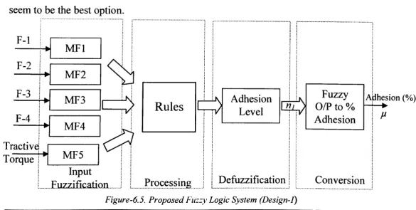
Figure-6.5. Proposed Fuzzy Logic System (Design-I) ...82
Figure-6.6. Variation in Residuals with the change in adhesion level ...83
Figure-6.7. Membership function for the residual of filter-1 ...83
Figure-6.8. Membership function for the Residual of filter-2...84
Figure-6.9. Membership function for the Residual of fllter-3... 84
Figure-6.10. Membership function for the Residual of filter-4...85
Figure-6.11. Membership function for the Measured Tractive Torque ...85
Figure-6.12. Output Membership function ...86
Figure-6.13. Defuzzified output vs adhesion level ...87
Figure-6.14. Data fitting process ... 87
Figure-6.15. Creep Curves ...88
Figure-6.16. Fuzzy Logic output on creep curve CA ...89
Figure-6.17. Tractive Torque Controlled by PI controller ...89
Figure-6.18. Fuzzy Logic output on creep curve CB ...90
Figure-6.19. Fuzzy Logic output on creep curve Cc ...90
Figure-6.20. Fuzzy Logic output on creep curve Cj ...92
Figure-6.21. Tractive torque to drive wheelset on Cj ...93
Figure-6.22. Fuzzy Logic output on creep curve Ci ...94
Figure-6.23. Tractive torque to drive wheelset on Cj ...94
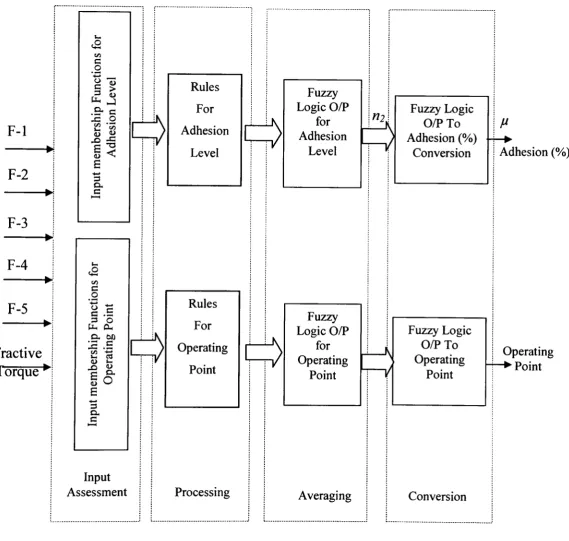
Figure-6.24. Fuzzy Inference System (Design-II) ...95
Figure-6.25. Basic Idea of Design-II ...96
Figure-6.26. Creep Curves for fuzzy inference system design ...96
Figure-6.27- Variation of Residuals of all filters on Ca ...97
Figure-6.28. Variation of Residuals of all filters on Q, ...97
Figure-6.29. Variation of Residuals of all filters on Cc ...98
Figure-6.31. Variation of Residuals of all filters on Ce ...99
Figure-6.32. Variation of Residuals of all filters on Cf ... 100
Figure-6.33. Variation of Residuals of all filters on Cg ... 100
Figure-6.34. Variation of Residuals of all filters on CH ... 101
Figure-6.35. Variation of Residuals of all filters on Q ... 101
Figure-6.36. Membership function of residual of filter-1 ... 102
Figure-6.37. Membership function of residual of filter-2 ... 102
Figure-6.38. Membership function of residual of filter-3 ... 102
Figure-6.39. Membership function of residual of filter-4... 103
Figure-6.40. Membership function of residual of filter-5... 103
Figure-6.41. Membership function of Tractive Torque ... 103
Figure-6.42. Membership function of Residual of filter-1... 104
Figure-6.43. Membership function of Residual of filter-2... 104
Figure-6.44. Membership function of Residual of filter-3 ... 105
Figure-6.45. Membership function of Residual of filter-4 ... 105
Figure-6.46. Membership function of Residual of filter-5 ... 105
Figure-6.47. Membership function of Tractive Torque ... 106
Figure-6.48. Output Membership function for Adhesion level ... 108
Figure-6.49. Output Membership function for operating point ... 109
Figure-6.50. Simulation Result when the wheelset is operated on Ca ... 109
Figure-6.51. Simulation Result when the wheelset is operated on Ca ... 110
Figure-6.52. Simulation Result when the wheelset is operated on Ca ... 110
Figure-6.53. Simulation Result when the wheelset is operated on Ca ... 111
Figure-6.54. Simulation Result when the wheelset is operated on Q, ... 111
Figure-6.55. Simulation Result when the wheelset is operated on Cg ... 112
Figure-6.56. Simulation Result when the wheelset is operated on Cj ... 112
Figure-6.57 Simulation Result when the wheelset is operated on CK ... 113
Figure-6.58. Simulation Result when the wheelset is operated on Ch ... 113
Figure-6.59. Simulation Result when the wheelset is operated on Cc ... 114
Figure-6.60. Simulation Result when the wheelset is operated on Cd ... 114
Figure-6.61. Simulation Result when the adhesion level is changed from Ca to Cd ... 115
Figure-6.62. Simulation Result when the adhesion level is changed from Cg to Ca ... 116
LIST DF TABLES
Table-5.1: Residual Values for Design I ...63
Table-5.2. Residual Values for Design II ...76
Table-6.1: Fuzzy Logic Rules forDesign-I ...87
Table-6.2: Fuzzy Logic Rules for adhesion level ... 107
1. INTRODUCTION
1.1 Introduction
Since the beginning of rail travel, adhesion between the wheel and the rail has been a crucial parameter in the design and operation of the railway vehicles, particularly during the autumn leaf falls, when the leaves are crushed to form a low-adhesion contaminant film on the rail surface, which is extremely difficult to remove. Poor adhesion can either be caused by naturally occurring weather conditions or the local environmental or industrial conditions. Some of the causes, such as leaf contamination, snow, ice, oil spills, etc., may be obvious and well known, while others such as industrial pollutions are not so obvious. However, they all have a similar effect in that they reduce the level of adhesion.
Figure-1.1: Contaminants on railway tracks
suffer from wheel burns and deterioration caused by damaged wheels. Wheelsets then need re-profiling or replacing and the rails need regrinding, thus causing additional costs to the rail industry. Furthermore, there is loss of train availability during the period of repair [1]. Wear due to wheel slip/slides and disruption to train schedules is the most important aspect from an economic perspective. However, from the safety point of view, when the friction levels are very low a train might not be able to brake within the available distance, making this aspect of even higher importance. Extremely low friction values between the wheel and the rail have been reported worldwide, leading to severe delays and sometimes even to accidents.
- - -^ y&t
V^ i ****&$& j* KL^'^T~*'"^J ^- "
1Ss>iSr / jaaRs'SS'- i^floe*' riS.r-'*^
^i.-',^- x n* «^-" *-i"-'^f..^^r ^^v" "^^^c:..''
•1t%H%K^^.VS»f§*?^f jkJ^S-S*?"^ ^i'^^-'^C^.^W -^S^??*jTjf?>»l *^t<'»4«i-*i.W > y^i/^X;^^
T^XVX.^-A:,'^ ^^£s"''A^\H
LA „.«» • fc v.'Ji ,» .
.. * K.-i^»o5r ^.*i '
Figure-1.2: Damaged track after severe wheel slip
Another side effect is that it tends to influence the behaviour of the driver. Basic knowledge about low adhesion is limited and based largely on subjective observations offered, for the most part, by drivers. Therefore it is up to the drivers, and because they shoulder great responsibility, they tend to be overly cautious on the basis of their 'feeling' concerning the condition of the track. When one driver encounters a slippery track during braking or accelerating, he may immediately communicate to other drivers that they ought to exert caution [2], Of course, such behaviour is "over-safe' when the friction levels are at acceptable limits, leading undoubtedly to delays and wasted drive time.
Dutch train operator NS-Reizigers suffered flat wheels due to excessive sliding, leaving thousands of travellers stranded overnight on their way home. In the following week, thorough maintenance was carried out on the rolling stock, but the lack of available train carriages made it impossible for the operator to run on schedule [2]. Low adhesion costs the railway industry significant sums of money each year, not only for various railhead treatments to minimise the occurrence of low adhesion conditions, but also for reduced operational performance and for the repair of wheels and rails where railhead treatments are not successful. According to adhesion working group (AWG) reports, the annual cost of low adhesion to the UK's rail industry as a whole exceeds £50 million [2, 4]. A large number of measures have been developed; nevertheless, the problems caused by low adhesion still persist.
For at least 150 years, research has been conducted on how to improve the transmission of power. The need for faster, more efficient and safer transportation over the past decade has made it increasingly important to improve the transmission of force. As a result, NS (the largest train operator in the Netherlands) and ProRail (Dutch infrastructure management company) have initiated the low adhesion research programme AdRem (Adhesion Remedy) [5]. The railway industry in the UK is currently taking formative steps in using the real-time condition monitoring of railway vehicles [6- 7], several techniques for which have been proposed, with the main emphasis on detecting areas of low adhesion as the train travels along the track [6, 8-11]. These condition monitoring techniques rely on available measurements, estimates and observations of the required parameters (such as creep forces) during normal running conditions of railway vehicle.
1.2 Motivation, aims and objectives of the study
The problem of low adhesion costs the railway industry significant amounts of money each year and raises several safety and reliability issues. Although in last few decades the railway industry has been able to manage low adhesion to some extent, currently available measures are not sufficient to eliminate safety incidents and train delays. Over one million scientific publications have been produced by researchers around the world alluding to this subject, including topics such as material technology, organic chemistry, rolling stock technology (also braking techniques, control techniques, traction installation), transportation processes, driver behaviour, safety, infrastructure, signalling systems, timetables, tribology, the dynamic behaviour of trains, weather and measuring techniques [5, 12]. Nevertheless, this volume of work has not resulted in an acceptable reduction in the problem, mainly because adhesion varies continually.
The wheel slip/slide phenomenon and associated damages and repair costs will be a thing of the past. The technique will also save time because the train will be driven more efficiently at speeds associated with the maximum use of available adhesion rather than using the current guidelines. It will also have a great impact on the quality of service in terms of passenger ride comfort and noise levels.
1.3 Railway vehicle dynamics
Wheel-rail contact conditions and the level of adhesion also play a significant part in the dynamic properties and behaviour of railway vehicles, especially those pertaining to wheelsets. The focus of this thesis therefore centres on the dynamics of the most fundamental element of railway transport vehicles, namely the wheelset. Railway wheels are different from the wheels on road vehicles in that both wheels are mounted rigidly on a common axle, the whole arrangement being known as a wheelset. There are exceptions, such as the Spanish high-speed train, the Talgo Express, which has independent wheels (as do many rail vehicles used in coal mines), but most conventional rail vehicles use the solid axle wheelset [13-15].
Wheel Flange
Axle
RaiL Figure-1.3: Railway Wheelset
non-zero speeds. This type of motion, when the wheelset moves in oscillatory form, is known as 'hunting', a problem which has been known to railway engineers since the very early days, although with very little scientific understanding at that time [13]. It is only in about last fourty years that an adequate theory for hunting has been available for vehicle suspension designers to use. One of the solutions to avoid hunting is by means of yaw stiffness, but choosing a suitable yaw stiffness value is another problem, as low stiffness limits the maximum speed of the vehicle and high stiffness degrades the curving performance of the wheelset. Another important factor that affects wheelset dynamics is the adhesion level during wheel-rail contact.
Creep
Figure-1.4: Adhesion coefficient vs. creep, representing different contact conditions
The contact between wheel and track is fundamental to railway operation. All the forces supporting and guiding the railway vehicle are transmitted through the contact patch, which is very small (about 1cm2) compared to its overall dimensions and shape. One of the most important factors in the transmission of these forces is adhesion level at the wheel-rail contact patch. However, the relationship between these forces and adhesion is very complex and depends upon the concept of creep, a phenomenon that occurs due to the elastic behaviour of the material at the wheel-rail contact patch.
proper traction and braking performance, a minimum level of adhesion (typically 0.25 for traction and up to 0.1 for braking) is required. In poor contact conditions, the maximum adhesion available can be far below what is needed for the normal provision of traction or braking.
1.4 Thesis structure
This thesis consists of seven chapters. In this chapter the problem of low adhesion in railway vehicles is described briefly. The basic operation of the solid axle railway wheelset and the effect of contact conditions on the dynamics of the wheelset are also described briefly.
In Chapter 2, the literature review gives a comprehensive introduction to the importance of adhesion in line with the traction and braking performance of the vehicle. The causes of low adhesion and its consequences on the performance of the vehicle are presented in detail. Later, the measures taken by railway operators around the world to improve adhesion are discussed in detail. Conventional wheel slip/slide protection techniques are also covered. Finally, the use of model-based estimation for railway condition monitoring is discussed. Based on the literature review, a brief conclusion is drawn to support the importance and approach of this research.
In Chapter 3, wheelset dynamics are discussed and a comprehensive mathematical model of a single solid axle wheelset is developed. In order to provide a better insight of complex wheel-rail mechanics the dynamics of the wheelset are analysed using various methods (Eigen value analysis, root locus, etc.) at different speeds and in different contact conditions.
In Chapter 4, simplifications in the wheelset model are introduced in order to simplify the design of the estimators. The design detail of the Kalman filter is presented and preliminary estimation results are presented to show the working of Kalman filters in different contact conditions.
In Chapter 6, basic idea of the fuzzy logic reasoning is presented. Then a brief introduction to the fuzzy inference systems is presented. Design of the fuzzy logic-based decision making systems for Design-I and Design-II are discussed in detail (including choice of type fuzzy system, type of membership functions and choice of deruzzification method). In the end, simulation results are presented for Design-I and Design-II to show the potential of this research.
2. LITERATURE REVIEW
The railway wheelset is a very complex mechanical system, its dynamics are influenced by many factors and uncertain variations in the contact condition make it even more complex. This chapter provides a literature review of the modelling and dynamics studies that have been carried out previously by other researchers. More relevantly, adhesion, factors affecting adhesion, solutions and proposed solutions for improvements based on previous research findings are detailed.
2.1 Railway wheelset modelling and dynamics
still increased, wheel macro-slip takes place and increases [25]. Wheel macro-slip can be avoided by means of an appropriate braking and traction control system.
2.2 Adhesion and adhesion management
A train is driven as a result of traction on the contact patches between steel wheels and steel rails. The advantage of using steel wheels on steel rails is low rolling resistance. This advantage, however, also poses a disadvantage: the wheel can only transmit relatively limited braking and traction forces to the rail. Therefore, the maximum values of traction are limited by the adhesion coefficient, known as the ratio of tangential force to the normal load [26]. Adhesion is one of the most significant factors influencing the dynamic response of the wheelset. The dynamic behaviour of a wheelset running on the railway track is governed by contact forces in lateral and longitudinal directions, which in turn are related closely to different contact conditions. In the last few decades, the railway network has been increasingly exploited, resulting in greater demand for faster services; consequently, the traction and braking capabilities of rail vehicles have been increased. However, the friction conditions between wheel and rail have not been improved, so the low adhesion problem remains a key issue in many railway networks around the world [25].
causes. On debris-free rails it acts as an additional boundary lubricant, while with debris present it forms a low shear strength mixture which, in minimally wet conditions, remains on the wear band where wheels contact the rail. In steady rain the debris mixture is squeezed aside and adhesion is possibly improved [30]. In dry weather, debris particles have apparently little influence on the overall adhesion coefficient. Oils on rails are present in minute quantities and are found to be complex mixtures containing an unusually high proportion of chemically active compounds. Laboratory experiments have studied how such oils and related compounds affect friction when present in surface concentrations similar to those found on the track [31]. Ever since the early days of railways, autumn leaves have been a source of disruption to train services in those areas where trees grow close to the trackside [37]. In the UK, train operations can be affected significantly during autumn leaf fall due to the resulting reduced adhesion, as the leaves are crushed to form a hard, slippery layer on the rail, which is extremely difficult to remove [8, 34, 38-39]. A typical variation of the adhesion coefficient with the relative wheel slip for dry and wet contacts is given in Figure-1.4.
Adhesion Related Incidents during autumn 2000 to autumn 2005 400
V) 1 300
20°
.£>
i 100
—••— Signals passed at Danger Station Overruns
2000 2001 2002 2003
Year
2004 2005
Figure-2.1: RAW Statistics on adhesion-related incidents
transmitted to the passenger part of the vehicle create discomfort in the ride. Extremely low friction values between the wheel and the rail also lead to severe delays and sometimes even to accidents. When viewed from a historical perspective, the risk from adhesion-related incidents can be characterised as high in frequency but low in consequence. There have been very few accidents arising from low adhesion, but the most significant occurred in November 1985, when two trains collided at Copyhold Junction in Sussex, resulting in 40 people being injured, 11 of them seriously [3]. In 1994, in the UK, nearly 600 adhesion-related incidents were reported including 91 signals passed at danger, seven buffer stop collisions, one collision with another vehicle and 503 stations overrun wholly or partially as the result of low adhesion conditions. Figure-2.1 shows the adhesion-related incidents from autumn 2000 to autumn 2005 reported by the Rail Accident Investigation Branch (RAIB). Railway industries around the world have suffered a great deal due to the problems caused by low adhesion.
are several other issues involved such as limited quantities of sandite available on board and the slower speed at which it has to be applied [3]. High pressure water jets were used in 1972 to remove leaf films from the rail surface [53-54], but the conclusion was that water alone was not effective at practical train speeds, although the monitoring of wheel flats on treated tracks suggested that some improvement in adhesion was attained [55- 56]. During 1974, a number of liquid systems were tested for their ability to increase wheel-rail adhesion when applied to the railhead by trackside applicators [57-58]. Network Rail, in the UK, applied sandite and water jets to eliminate low adhesion during the leaf fall season in 2005 [3]. There is an important distinction between the effect of water jetting and sandite, as the purpose of water jetting is to clean the railhead, whereas the purpose of applying sandite is to enhance adhesion at the wheel-rail interface. As such, in severe low adhesion conditions, sandite would be required in addition to water jetting [3]. Network Rail and its predecessor, performing the role of infrastructure manager for the national network, experimented with novel methods including surface scrubbing and laser cleaning. However, these methods proved to be impractical (lasers only work at very low speed and brushes wear out very quickly). Another problem in using a modifier is that it does not have exact information about the actual adhesion coefficient that sometimes results in excessive sanding and causes accelerated wheel wear and material waste damage to the track structure because of ballast fouling, drains and switch points, disruption to train detection systems and the premature rotting of ties. Certain commercial adhesion enhancers currently promoted involve rubbing a solid stick on the wheel, which leaves a layer of material on the wheel that comes in contact with the rail, therefore acts as a third layer and modifies friction between the two surfaces [44]. Although this approach improves friction in certain conditions, the extra layer of material left on the rails can have some negative effects on the non-tractive wheels.
braking and traction efforts as close to that maximum as possible [25]. WSP systems usually consist of two elements, one for detecting wheel slip/slide and another that has to be able to adjust traction and braking force [59]. The most common WSPs are developed by measuring the difference between the train speed and the wheel rotational speed [60- 61], and they rely on relative speeds measured by sensors that gauge the angular speed of the wheel and the absolute speed of the vehicle.
There are several practical issues involved in detecting these parameters. According to [62], the absolute speed of a train is normally obtained from a trailer bogie (or axle), but the provision of a reliable train speed is a problem when all the axles are affected, e.g. in braking. The requirement of robust/reliable sensors for what can be harsh working environments limits the accuracy of measurements. In a different research study, estimated vehicle speeds were used instead to improve performance in noisy mechanical environments [63], but conventional re-adhesion control techniques are not particularly sensitive to condition changes and only large variations tend to be detectable. Effectively, WSPs are reactive systems, i.e. only 'activated' to stop wheel slip/slide when detected by sensors. In some rail networks, LAWS (low adhesion warning system) or AMS (adhesion management systems) are used to provide estimates of track conditions based on a large pool of trackside measurements such as site topography, track geometry, microclimates and contamination. It is widely recognised that such localised adhesion conditions can be very beneficial to train drivers and to network operators, as they can take preventative measures and plan train journeys and schedules accordingly in order to maximise network capacity and efficiency within the constraints of the track conditions. Such systems are inevitably very complex and expensive to implement, and it is potentially difficult to deliver reliable estimates because of the large number of sensors that need to be installed across a network and the amount of data that must be collected and processed.
investigate the influence of basic parameters on adhesion [1]. It was concluded that the value of adhesion decreases as the axle load increases and that the influence of the curve is not significant. The National Traction Power Laboratory (NTPL), in China, undertook a detailed experimental investigation of the adhesion problem using a specially designed, full-scale roller rig with actual wheel and rail profiles [64]. The roller could not only rotate to simulate different train running speeds, but it could also vibrate independently in the vertical and lateral directions to simulate track irregularities. The adhesion coefficient was measured under water-contaminated, machine oil-contaminated, dry and clean surface conditions. British Rail (BR) Tribometer trains were also used to measure the longitudinal creep coefficients [135], which measures the relative longitudinal creepage between a braked and freely rotating wheelset. The actual brake force is determined via instrumented brake and suspension elements. A series of runs at various brake force levels gives a series of points on the creep curve.
Although various different experiments in the laboratory and on real tracks have attempted to prove the reliability of the measured value, there are several issues that need to be addressed such as roller rigs and Tribometer trains differing from actual trains in terms of axle load, speed and other important parameters that can affect the adhesion coefficient.
creep coefficient, have not been considered. In [67], a method for the identification of friction force is proposed. The identification is realised by means of observations carried out in the mathematical model of the physical system and of the driving motor. This method uses the derivative of the adhesive effort with respect to the slip velocity to determine the saturation point, which is difficult because the derivation of the slip velocity is highly sensitive to measurement noise caused by the limited resolution of practical speed sensors. In a similar work, the derivative of friction force is estimated to eliminate the problem of sensor resolution [68]. The derivative of friction force is estimated by means of a high-pass digital filter.
Another approach to re-adhesion control is based on disturbance observation [69], which estimates disturbance torque by using rotor speed and torque current information. However, the performances of anti-slip schemes based on a disturbance observer are affected to a large extent by noises in the system, which can be very substantial in the wheel-rail contact environment.
In recent research an indirect approach was used for wheel slip detection and explored changes in wheelset dynamics and in wheel-rail contact conditions [62, 70-71]. The study showed that torsional vibrations of specific frequencies (associated with material damping) in the axle are produced when creep forces are saturated. This finding provided an opportunity to develop a novel re-adhesion control technique that could detect axle vibrations of specific frequencies and hence wheel slip. Two detection methods proposed are running FFT to detect the spectrum variation of a particular frequency, while the other uses bandpass and low-pass filters to obtain magnitude information on the frequency of interest.
2.3 Condition monitoring
occurs. Monitoring can either be used to improve maintenance procedures for railway vehicles or to determine the current running conditions of in-service vehicles, without the use of cost-prohibitive sensors [6]. The generic railway condition monitoring system uses some level of knowledge of the system in the form of a mathematical model, expert system, learnt behaviour, etc. and measured outputs to perform its diagnosis, but unlike other condition monitoring applications the dynamic response of the system is driven by irregularities in the track, which are difficult to measure and therefore cannot be applied to a condition monitoring system [9, 74]. The use of condition monitoring techniques to identify local adhesion conditions along with other condition monitoring parameters has recently been adopted by several researchers. A number of ideas have been proposed to detect the running conditions of the wheel-rail interface [6, 9-11, 75-77]. A model-based scheme for condition monitoring at the wheel-rail interface is proposed in [9] whereby the adhesion level is identified by measuring the dynamic response of the vehicle to lateral track irregularities under normal running. This work is carried out further in [6, 78-81], with the primary aim to estimate creep forces generated at the wheel-rail contact. Estimating these forces has many applications such as local adhesion level estimation, the prediction of rolling contact fatigue, the prediction of wheel tread wear, the estimation of track damage caused by specific vehicles and potentially as a cost-effective method of assessing engineering design changes to wheel tread geometry. An inverse modelling approach for the estimation of creep coefficients, using measured car body acceleration, is proposed in [75-77]. There are also a number of other applications in railway vehicle research that used the interacting multiple model (IMM) algorithm for condition monitoring [21, 82-85]. In [83], IMM is used to detect and identify failures in suspension. In addition, multiple Kalman filters are used to describe different modes of suspension failure.
2.4 Model-based estimation
and accuracy in the presence of stochastic noises, provides an opportunity to estimate key vehicle parameters such as vehicle mass, tyre cornering stiffness, under-steer gradient, roll stiffness and the roll damping coefficient. Once vehicle parameters have been estimated precisely, parameterised vehicle dynamics models with properly estimated parameters can be used for a wide variety of applications including highway automation, vehicle stability control and rollover prevention systems [87-90]. The Kalman filter has also been used in a variety of rail vehicle applications such as actively controlled railway vehicle suspension, fault detection of railway vehicle suspension, low adhesion estimation and in re-adhesion control schemes to estimate important parameters
[8,14,83,91].
Adhesion between the wheel and rail varies stochastically and depending upon several factors. The Kalman filter has been applied successfully in various condition monitoring applications to detect adhesion variation [8-9], and [38] presents a Kalman filter-based estimation scheme to estimate the adhesion force coefficient. A half vehicle model, consisting of two wheelsets, one bogie and a half vehicle body, is used to simulate behaviour. The dynamics of the wheelset are modelled using linearised creep forces valid only in the low creep region of the creep curve. In [9], model-based condition monitoring at the wheel-rail interface is presented. Two applications of model based condition monitoring are proposed one for wheel-rail profile estimation and the other for low adhesion detection. A Kalman filter is used to estimate the wheel-rail profile and estimation is carried out on a linearised simulation model. In an indirect adhesion estimation method, the Kalman filter was used to detect slip [62]. Traction motor speed was used to estimate torsional oscillations, and the results showed that the Kalman filter provided a level of estimation sufficient for slip detection and it was robust in a variety of different slip conditions.
"residual') between the measured sensor values and the values predicted by the model embedded within the filter [94]. The model selection takes place based on the value of the residual signal. The multiple model-based estimation has also been used in railway vehicle research [21, 83, 85], especially in fault detection application where system parameters are changed over time. For example, in [21] a multiple model approach to detect faults in suspension using on-board measured data is proposed.
2.5 Fuzzy logic
There is a variety of vehicle dynamic applications in which the fuzzy logic is used, especially in automatic steering and intelligent control for vehicle systems in which the vehicle dynamics have various structured uncertainties and nonlinear characteristics. Not only are uncertainties unknown or poorly known, but they also may be subject to change as the vehicle goes about its navigation [95]. In such situations, the lack of information about parameters makes it difficult to design a conventional control scheme, so fuzzy logic is considered better suited for such types of application. Other applications include the use of logic-based control for the purpose of determining and assigning desired wheel slips for each corner of a vehicle [96], a fuzzy logic controller to control the lateral motion of the vehicle [97], yaw moment control based on fuzzy logic to improve vehicle handling and stability [98] and a fuzzy rule-based Kalman filtering technique for an accurate estimation of the true speed of a vehicle [99]. There are various railway vehicle applications where fuzzy logic is used either for estimation or for control [100-103], and [100-101, 103] present techniques based on fuzzy logic to control the steering and traction torque of the wheelset, while [102] presents fuzzy logic-based gain scheduling control for a nonlinear suspension system.
applications in which various models produce different sets of data. Therefore, some sort of decision-making system is required that can compare the actual result with the output produced by various models and identify the most valid model among several. Fuzzy logic is useful in circumstances where it is practically impossible to describe all the nonlinearities and changes in parameters using a multiple model-based system; therefore, fewer models are used to design the system, and the possible behaviours of the system are described using these fewer models.
2.6 Summary
The presence of contaminations on rails such as snow, water, oil, tree leaves etc. presents a serious challenge to traction and braking control systems. There is currently a paucity of knowledge regarding low adhesion and it is based largely on subjective observations, for the most part offered by drivers. Available techniques for railhead treatment are not sufficient to cope with the problems arising from low adhesion, and the absence of an adhesion measurement tool is the major reason why slippery tracks are still a problem. In order to make the current measures more effective, it is necessary to provide real-time information about track conditions as the train travels along the track. This will help traction and braking control systems (WSPs) to maximise the use of available adhesion and thus maintain the stable operation of the railway vehicle.
The dynamic response of the railway wheelset on any creep curve depends on the location of the operating point on the creep curve. As the operating point moves up and down due to the application of traction and braking forces, the dynamic response varies accordingly. Specifically the dynamic response of the wheelset at a particular operating point on any given curve depends upon the slope of the creep curve ( -) and on the traction ratio (
Y
design point. Increased estimation errors are expected if the contact condition is not at or near to the chosen operating point, while the level of matches/mismatches is reflected in the estimation errors (or residuals) of the models concerned, when compared with the real vehicle (through the measurement output of vehicle-mounted inertial sensors). A fuzzy reasoning procedure is developed to translate and map the estimation residuals from all the models into direct information on track conditions and adhesion levels, which in turn can be used by train drivers and network operators (or traction/braking control systems). All the simulations are carried out in the MATLAB/SIMULINK environment.
Slope = - =
dy
Traction Ratio = L
Y^
Jl
Figure-2.2. Basic concept of contact condition identification
two operating points. It is highly unlikely that two operating points can have the same slope, traction ratio and same amount of tractive effort. Therefore it is concluded that the contact condition may be identified by analysing the residuals and the tractive torque.
3. WHEELSET MODELLING
3.1 Railway vehicles
Railway vehicles employ steel wheels that run on steel rail tracks, which provide support and guidance functions. The interface between the two is established at contact point(s) between the wheels and the rail surface, and both the vehicle configuration and the track greatly influence how vehicles behave [109]. Figure-3.1 shows the configuration of the most modern passenger-carrying railway vehicles. Each car consists of two bogies, each of which has two sets of wheels. The purpose of the bogie is to carry the weight of a vehicle along the track at the required speed and with a high degree of safety. In so doing, and as far as practicable, it isolates the vehicle from dynamic forces and vibrations resulting from motion. The car body is connected to bogies via suspensions (secondary suspension), the purpose of which is to provide good ride quality by isolating the car body from vibrations induced by track irregularities. The wheelsets are connected to the bogie via primary suspensions, whose elements are much stiffer than in the secondary suspension system and are designed to satisfy the vehicle's stability and guidance requirements. The left and right side wheels in each wheelset are connected rigidly via a common axle (known as the solid-axle wheelset) such that the two wheels have to rotate at the same speed.
a
Car BodySecondary Suspension
\
Primary Suspension
Bogie | Frame Wheelsets
Figure-3.1: Railway vehicle configuration
with the track. Therefore, a single solid axle wheelset is considered in this study. The dynamics of the bogie do have some effect on the wheelset dynamics but the end result is not too different from single wheelset and also in various other stability and guidance studies the primary focus of the study has been on a single wheelset which can be easily extended to two axles and a full vehicle with some modifications [9, 14, 17-20, 23, 31, 70-71, 110-111]. The simplified plan view of the wheelsets in a bogie frame is shown in Figure-3.2. The single solid axle wheelset consists of two wheels connected rigidly to an axle (hence the name 'solid axle wheelset'). The wheels are considered as two rigid cones, although in practice they are of a profiled structure. The flanges are a necessary precaution and they should never touch the rails except on sharp curves to meet an accidental, lateral force [112].The coned tread helps the wheelset to maintain a pure rolling motion in a curve, if it moves outward and adopts a radial position [15].
1
Figure-3.2: Railway wheelsets in a bogie frame
analysis of kinematic oscillation [113] and derived the relationship between the frequency/and the wheelset conicity ^w , wheel radius r0 and the lateral distance between the contact points between wheels and rails 2Lg as [15].
(3.1)
Figure-3.3: Railway wheelset slightly displaced in the lateral direction
The wheelset is connected to a vehicle body or bogie via suspension elements set in lateral and longitudinal directions. The longitudinal connections between the wheelset and the bogie are assumed to be solid, as the stiffness is normally very high and associated dynamics are not of significant relevance to this study [114]. The lateral springs are necessary to transmit the curving forces, so they are therefore not considered for further study, as in this thesis only a straight track is taken into consideration.
Figure-3.4 shows a wheelset running on a straight track. The coordinate system
oxyz moves synchronously with the wheelset at the speed of the vehicle, while origin O
is constrained along the centre line of the undistorted track. The jc-axis points along the rails in the rolling direction are also known as the 'longitudinal direction', and they-axis (lateral direction) is a 90° lag to complete a right-hand coordinated system. The z-axis points vertically upwards. The yaw angle (*//„) is the angular displacement around the vertical axis.
3.2 Creep and creep forces
Creep is said to exist when a wheel deviates from pure rolling, that is the distance covered by the wheel in one revolution is not equal to the circumference of the wheel. Pure rolling rarely takes place, and wheels and rails are not rigid [115]. The normal load between the wheel and rail causes local elastic deformation, and an area of contact, the contact patch, is formed. In the contact patch the material is compressed at entry before a section where adhesion takes place then a section where the material slips out of compression and finally exits in tension [19]. Creep is defined as the relative speed of the wheels to the rail and is characterised as lateral and longitudinal creep in accordance with the direction of motion. If a longitudinal force is applied to the wheel, a deviation from the pure rolling motion occurs. The deviation in relative velocity, divided by the forward speed of the wheel, is referred to as longitudinal creep (yx ) [116].
where vv is the vehicle's forward speed and v w the equivalent linear speed of the wheel, which is given by
vw=*V (3.2)
VH•R = ®WR • \T0 - 4 (yw - yt)] (3.4)
where ft)wL is the left wheel's angular speed, 6)wR the right wheel angular speed, r0 the radius of each wheel when the wheelset is running in a centre position, Aw the wheelset conicity and y t the disturbance applied by the track in a lateral direction. Usually there are four inputs to the vehicle from the track: vertical profile, cross level, lateral alignment and gauge [13], but only lateral disturbance is considered here because of its direct effect on yaw and lateral dynamics. Irregularities in the gauge are very small as compare to y, therefore, are not considered in this study. Yaw movement will also contribute to the longitudinal creepage in opposite directions for the two wheels [70]. Creepage for the left (yxL ) and right (yxR) wheels can then be written as
-vv
V V V V VV
*
*
,
V V V V VV
where Lg is the track's half gauge, y/w the yaw angle of the wheelset and yw the lateral motion of the wheelset. When a wheelset is displaced laterally, yaw torque steers the wheelset against the restraining effect of the suspension. If a wheelset is forced to run at an angle of attack to the rails, lateral creepage (yy ) is produced [13], which is defined as the relative lateral velocity divided by the forward speed [115].
vV
(3.7)
Spin creepage has an important value when flanging [19], but in this study flange contact is not taken into account. The total creepage for each wheel is given by
(3.8)
Y (3.9)
Figure-3.5 shows a typical nonlinear variation of the adhesion coefficient with creep. The creep curve can be divided into three regions to describe the stable and unstable behaviour of the wheelset. The initial part of the curve is linear and a low creep section, in which almost the entire contact area is occupied by the non-slip region; the wheelset operates in this region when the vehicle is operating in steady conditions. With the increase in tractive effort, the slip region at the wheel-rail contact patch increases and the non-slip region decreases. When the tractive force reaches its saturation value, the non- slip regions disappear and the entire contact area is in a state of pure sliding.
.2n
'o
o
o Nonlinear
Unstable 'Slip )Non-Slip
Creep
Figure-3.5: Creep vs. adhesion coefficient
FxL
Figure- 3.6: Creep forces at the contact patch
3.2.1. Creep forces
called creep forces and occur due to micro-slippage or creepage in the area of contact [19]. The relationship between creep and creep forces has been studied thoroughly by Kalker [117] and his equations are widely used in simulations. The following figure illustrates creep forces generated at the contact patch.
The forces between the wheel and rail due to creepage are of fundamental importance to the dynamic behaviour of railway vehicles because they are widely recognised to present nonlinear characteristics as a function of creep, as shown in Figure- 3.7. In normal running conditions where creep is small (area before JUL in Figure-3.7), the contact forces provide a damping effort to the dynamic modes of a wheelset and are very useful in stabilising those modes, which would otherwise be almost critically damped. In this case there is adhesion over the complete contact area (according to the Hertz theory) and there is a linear relationship between creep forces and creepage [15]. This is in the form
FX =fu7X J = L,R (3.10)
where /H and /22 are creep force coefficients and represent the slope of the creep curve at the operating point of the wheelset. As creep increases, contact forces can operate in the nonlinear region (between fiL and //^ ), where the rate of change of the creep forces and their associated damping effect is much lower. For large creep sections of the creep curve, the representation of creep forces in longitudinal and lateral directions for the left and right wheels is given in the following equations:
YR
-t - r ——— -i 7 « ———————— * * ——— Xm. I/ /*"> 1 ^> \
'L L YL (3 ' 13)
where F^ , FxL , FyR and F L are creep forces in longitudinal and lateral directions for the right and left wheels respectively, and FR and FL are total creep forces for the left and right wheels at the wheel-rail contact patch and are a function of the adhesion coefficient (//) and normal force (N ).
o
o [t.
ex
<u
<u
U
max
Creep (/ =
Figure-3.7: Creep vs. creep force
When creep is beyond the point of the maximum adhesion available (/^x in Figure- 3.7) at the wheel-rail interface and enters the slip and unstable region, contact forces will then become a destabilising element, which not only causes the well-known problem of wheel slip (in traction) and slide (in braking), but also can lead to other undesirable mechanical oscillations in the wheelset.
3.3 Wheelset dynamics
It is essential in the study of wheelset dynamics to develop and use a comprehensive model that includes all relevant motions related to the contact forces, because strong interactions between different motions of the wheelset through creep forces during wheel-rail contact act in both the longitudinal and lateral directions. In this section a comprehensive wheelset model is introduced, which considers all the relevant motions. A single solid axle-powered wheelset is considered for basic study, with a traction motor mounted on the right side of the wheelset. Therefore, traction torque (Tt ) is applied directly to the right wheel. It is assumed that the normal load on either side of the wheelset is the same. Railway wheelset has several degrees of freedom. The lateral displacement and the yaw angle are two small movements relative to the track. The displacement along Ox and the rotational motion around Oy are determined by longitudinal speed vv . The rolling radius r of the wheel, the wheelset centre of gravity height z and the roll angle around Ox are linked to rails when there is contact on both rails [109]. The longitudinal motion of the wheelset is a result of left and right wheel creep forces in the longitudinal directions.
= XR+ xL (3.15)
^ = F*Lg - FxLLg - k^w (3.16) where Iw is the yaw moment of inertia and k» is the stiffness of the yaw spring that connects the wheelset with the bogie. When the wheelset is moved in the lateral direction, one of the wheels has greater contact radius than the other, which introduces a small roll motion, the roll motion formulated as [19].
(3.17)
LLg
Lateral dynamics are determined by the total creep force of the two wheels in the lateral direction.
jl = ~FyK ~FyL +Fc +Fg (3.18)
where Fc is the centrifugal force which is taken into consideration when the wheelset runs on a curved track (given in equation (3.19)) and Fg is a gravitational stiffness force depending on the lateral displacement and roll angle of the wheelset [19] (given by equation (3.20)).
F
=^-Fg =~m ^=-3 (3.20)
Lg
Rc in equation (3. 19) is the radius of the curve. The wheelset is driven by the traction motor mounted on one side (the right side in this case) of the wheelset. The other wheel is driven by torsional torque transmitted through the axle.
IR^R= Ti - Ts- TR (3.21)
IL**L=T,-TL (3.22)
where Ts is torsional torque and TR and TL are the tractive torques of the right and left wheels respectively. The torsional torque along the shaft is determined by the difference in rotation between the two wheels [70]:
T =
--[-
• + •(3.24) +
I..W... =
• + •
V
--[:
• + •(3.25) • + •
—-¥,
V V V V VV
(3.26)
(3.27)
where 9. =
|
,.
v V v V vV
(3.28)
Longitudinal Creep Left Wheel
Longitudinal Creep Right Wheel
0
Figure-3.8: Simulink model of nonlinear wheelset dynamics Creep Curves
0 0.01 0.02 0.03 0.04 0.05 0.06 0.07 0.08 Creep
Yaw Angle
0.02-TD (0
-0.02-Lateral Motion
(A
0.04 r
0.020.02
--0.04 h
8 10
246 Time (Sec)
Figure- 3.10: Step response of an unconstrained solid axle wheelset at 20m/s
When yaw stiffness is provided to the wheelset, the yaw and lateral dynamics are stabilised for range of speed values, depending upon the amount of stiffness provided. Figure-3.11 demonstrates this phenomenon when the wheelset is operated at 20m/sec with yaw stiffness.
x 10-3 Yaw Angle
x 10-3 Lateral Motion
C/5
o>
•s
^
o 6 4 2 0
r ——————— L L i L
!
———
—— 1 r r r r
0 4 6
Time (Sec)
8 10
x 10-3 Yaw Angle
c
- 1
TD ' (0
0
-1
0 8 10
8
6
CO
I 4
x 10-3 Lateral Motion
4 6
Time (Sec)
8 10
Figure-3.12: Step response of a constrained solid axle wheelset at 60m/s and Kw=5*106N/rad
Figure-3.12 and Figure-3.13 show the results of yaw and lateral dynamics when the wheelset is operated at the same speed and with different yaw stiffness. In Figure-3.12 the yaw stiffness is higher, so the wheelset dynamics are stable at a higher speed (whereas, in Figure-3.13 with a less stiff spring, the wheelset is unstable at higher speeds). Nonetheless, the problem with high stiffness is that it degrades the natural curving ability of the wheelset.
0.2 r
Yaw Angle
Lateral Motion 0.2 r
4 6
Time (Sec)
8 10
9000
80007000
6000
-
5000-
4000-
3000-
2000-
1000-Tractie Torque
10000
5000--5000
32
r—r-o
<U
2 30
28
! 3 4 5 6 7
Time (Sec)
Figure-3.14: Applied tractive torque
Torsional Torque
456 Time (Sec) Vehicle Speed
456 Time (Sec)
8
8
8
10
10
10
Figure-3.15: Wheelset dynamics in different contact conditions
stiffness and material damping of the axle, as shown in Figure-3.15. Because of the slip the speed of the wheels increases abruptly (Figure-3.16), causing the mechanical parts of the rolling stock to wear down quickly and waste of power, whereas the increase in vehicle speed is much slower (Figure-3.15) because of the wheel slip.
200
o 150 o>
en
2 100
50
200 r
o 150-<U
CO
=0
2 100 h
50 ^^
Left Wheel Angular Speed
1 23456789 10
Time (Sec)
Right Wheel Angular Speed
1 23456789 10
Time (Sec)
4. ESTIMATORS DESIGN
4.1 Simplification of wheelset dynamics
The main objective of this study is to develop a new model-based technique to detect changes in wheel-rail contact conditions by using the least number of on-board sensors. One of the major steps in doing so is to estimate the wheelset dynamics in different contact conditions. For practicality purposes, it is necessary that the design of the estimators should be as simple as possible by considering those wheelset dynamics related directly to contact conditions. Previous studies have shown that lateral and yaw dynamics are sufficient to detect these changes [8-9, 14, 118-121]. Therefore, some simplifications in the wheelset model are introduced for the estimator design. The simplified equation of creepage involving only yaw and lateral dynamics is given below. The longitudinal creep of the left wheel is given in equation (4.1).
T ^ + ^Myw -y,)
(4.1)
v _
ixL ~
v,.
where = - - = .As such, equation (4.1) is rewritten as
v.. v. r
v
-7xL - (4.2)
v
Right wheel longitudinal creep and lateral creep are given in equations (4.3) and (4.4) respectively.
v
fxR (4.3)
7 ~
v,.
The simplified equations of lateral and yaw dynamics can then be written as:
+ Yyl
• + •
V
Ls-v,,
(4.4)
(4.5)
(4.6)
—
-vv
v,, V
(4.8)
•\JYxR + YyL
The simplified model has several advantages in estimator design, without having a significant effect on the results [119-121]. The major advantage is the simple design of the estimator with a minimum number of states that allow the estimator to converge quickly. The yaw and lateral dynamics are excited by lateral track irregularities; hence, torque input is not required for the estimators in the simplified model.
4.2 Linearisation of creep forces
In equations (4.5 and 4.7) creep forces FXR, Fxi, FyR and Fyi have a nonlinear relationship with creepages yx and yy. Therefore, these creep forces are linearised at specific operating points on the creep curve in order to design the Kalman filters. The first order approximation of longitudinal creep force for the right wheel around an operating point
yyRo) is given in the following equation:
(4.9)
F - F &• - F
2 xR ~ 2 R- ~ L
xR
where
dF,xR
xR ** R ^YlR~-' "2
(4.10)
Placing FR = juRNR into the above equation and considering = gives
dF,xR
xR (?xRo ' YyRo
)
R
(4.11)