Sensorless Control of a Linear Compressor Using Motor Parameter Identification

(1)

International Journal of Emerging Technology and Advanced Engineering

Website: www.ijetae.com (ISSN 2250-2459,ISO 9001:2008 Certified Journal, Volume 5, Issue 6, June 2015)

257

Sensorless Control of a Linear Compressor Using Motor

Parameter Identification

Gyu-Sik Kim

1

, Joon-Tae Oh

2

1_{The University of Seoul,163 Seoulsiripdae-ro, Dongdaemun-gu, Seoul, 130-743, Korea} 2_{Seoul Metropolitan Rapid Transit Co. Ltd., Seoul, Korea}

Abstract— The closed-loop sensorless stroke control

system for a linear compressor has been designed. The motor parameters are identified as functions of piston position and motor current. They are stored in a read-only memory table and used later for the accurate estimation of piston position. In addition, it is attempted to approximate the identified motor parameters to the second-order surface functions. In this study, we improved the results in [14]. PIM III algorithm is also proposed and the performances of PIM I, PIM II, and PIM III whose indices are memory size and computational time are fully evaluated. Some experimental results are given in order to show the feasibility of the proposed control schemes for linear compressors.

Keywords—Sensorless stroke control, Linear compressor, Estimation of piston position, Identified motor parameters, Second-order surface function

I. INTRODUCTION

A conventional reciprocating compressor uses a crank mechanism in order to change the rotational motion of a motor into linear motion. Accordingly, a reciprocating compressor can be operated safely by virtue of the crank mechanism, even though it makes the reciprocating compressor less efficient. However, the moving parts of a linear compressor are not constrained. Thus, the implementation of a closed-loop control system is necessary for the accurate control of piston position.

It was shown that linear compressors had extremely low friction losses compared to other compressor types and high efficiency could be achieved for a variety of refrigerants and compressor sizes [1]. The problems associated with the linear motor configurations which are potentially applicable to linear compressors were discussed [2]. They described moving coil type and moving magnet type linear motors and two methods of the linear compressor control that had been successfully applied. Some non-refrigeration applications for linear compressors were also studied [3]. A small linear compressor which operates at 50Hz was designed for the european market which could serve a variety of small and portable coolers for specialty uses, including recreational or medical cooling [4].

The piston positioning accuracy and the efficiency of the sensorless linear compressor system with the linear pulse motor were examined using analytical and experimental approaches [5]. But, the motor parameters were not identified fully. A dual stroke and phase control system was proposed for linear compressors of a split-stirling cryocooler [6]. A linear compressor was developed for 680 liter household refrigerator [7]. It reduced the energy consumption of a refrigerator by 47% compared with a reciprocating compressor. In [8], they showed that LGE created the innovative linear compressor, which has much higher efficiency in the small cooling capacity. The refrigerator with this linear compressor shows that the power consumption reduction by 25% can be achieved, as compared with the reciprocating compressors.

(2)

International Journal of Emerging Technology and Advanced Engineering

258 The performance of linear compressors using a pulse width modulation inverter is investigated, with emphasis on the efficiency and power factor along with variations of both mechanical and electrical resonant frequencies [12]. In [12], the strategy for improving the efficiency of the linear compressor was suggested by controlling the average value of the product of the piston stroke and motor current to 0. The mathematic model of the self-sensor was established by analyzing the moving magnet linear motor of linear compressor, and the measurement method of piston stroke was achieved [13]. In [13], the piston stroke can be calculated by measuring the voltage and current of the linear motor coil.

The closed-loop sensorless stroke control system for a linear compressor has been designed. The motor parameters are identified as functions of piston position and motor current. Then, they are stored in a read-only memory (ROM) table and used later for accurate estimation of piston position [14].

In this study, we improved the results in [14]. PIM III algorithm is also proposed and the performances of PIM I, PIM II, and PIM III whose indices are memory size and computational time are fully evaluated by experimental studies.

II. SENSORLESS CONTROL OF LINEAR COMPRESSOR

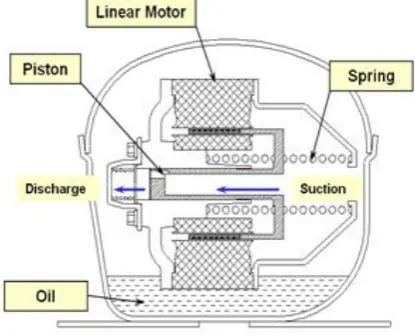
The mechanical structure of the linear compressor studied in this research is shown in Fig. 1. The equivalent electrical circuit of a linear motor in a linear compressor can be modeled and expressed as the linear differential Eq. (1). The thrust force Fe (t) is expressed in Eq. (2).

𝛼𝑑𝑥(𝑡)_𝑑𝑡 + 𝐿𝑒𝑑𝑖(𝑡)_𝑑𝑡 + 𝑅𝑒𝑖(𝑡) = 𝑉(𝑡) (1)

[image:2.595.328.536.142.310.2]

𝐹𝑒(𝑡) = 𝛼𝑖(𝑡) (2)

Fig. 1. Mechanical structure of a linear compressor.

Since the magnetic flux density varies depending on the piston position, the force constant and the effective inductance are functions of the piston position. The effective resistance is assumed to be constant because its variance, being negligible, is ignored. ( ) is the applied voltage to the linear motor, ( ) is the current flowing through the winding coil, and ( ) is the piston position. However, the mechanical equation of motion can be described as:

𝑑 𝑥(𝑡)

𝑑𝑡 +

𝑑𝑥(𝑡)

𝑑𝑡 + (𝑡) = 𝛼𝑖(𝑡) (𝑡) (3) Where , , and denote the equivalent mass, viscous damping coefficient, and spring constant, respectively. is the cross-sectional area of the piston, ( ) is the pressure difference between the compressor chamber and the back surface of the piston.

Taking the Laplace transform of the above Eqs. (1–3) yields:

( ) = ( )𝑉( ) + ( ) ( ) (4) ( ) = ₍₎ ₍ ₎ (5)

(3)

International Journal of Emerging Technology and Advanced Engineering

259 A closed-loop linear compressor control system needs piston position information. In order to measure the piston position, an inductive position sensor, in which the inductor is a small stationary coil wound on a ferrite coil, can be used. However, this position sensor is more expensive than a current or voltage sensor. It is also hard to install a position sensor in a linear compressor. Hence, it is more desirable to estimate the piston position indirectly. Rearranging Eq. (1), one obtains:

𝑑𝑥(𝑡)

𝑑𝑡 =

1

(𝑉(𝑡) 𝐿𝑒𝑑𝑖(𝑡)_𝑑𝑡 𝑅𝑒𝑖(𝑡)) (7)

The estimated value of the piston position can be obtained by integrating Eq. (7):

̂(𝑡) = ∫ (₀𝑡 𝑑𝑥_𝑑𝜏) 𝑑𝜏

=1∫ [𝑉(𝜏) 𝑅₀𝑡 𝑒𝑖(𝜏)]𝑑𝜏 𝑖(𝑡) (8)

For a digital control system, ̂( ) can be modified to digital form as

̂(𝑛) =𝑇 𝛼∑ (

𝑉(𝑘 1) + 𝑉(𝑘)

2 )

𝑛

𝑘=1

𝑇𝑅𝑒

𝛼 ∑ (

𝑖(𝑘 1) + 𝑖(𝑘)

2 )

𝑛

𝑘=1

𝑖(𝑛), 𝑛 = 1,2,3,∙∙∙∙ (9)

Where is the sampling period.

In general, the stroke is defined as the distance between the top and bottom piston positions during one cycle of operation (i.e., the peak-to-peak value of piston position). Therefore, the estimated stroke can be easily calculated using the estimated piston position. Let a phase delay filter ( ) be defined as:

𝐻𝑑( ) =2𝜋𝑓−𝑠_{2𝜋𝑓 𝑠} (10)

Where is the running frequency of the piston. If ̂ ( ) is assumed to be the phase delayed output of ̂( ), then the estimated stroke ̂( ) can be calculated as

̂(𝑡) = √ ̂2_{(𝑡) + ̂}

𝑑2(𝑡) (11) Fig. 2 shows the block diagram of the closed-loop sensorless stroke control system for a linear compressor. The applied voltage ( ) and the motor current ( ) are measured and input to the digital signal processor (DSP)

central processing unit (CPU) chips after

[image:3.595.56.538.156.354.2]

analog-to-digital (A/D) conversion. These measured variables, together with motor parameters, are used to estimate the piston position as shown in Eq. (9). The estimated stroke ̂( ) is compared with the set-point value of the stroke ( ) which is determined depending on load conditions.

(4)

International Journal of Emerging Technology and Advanced Engineering

260 The output of the proportional–derivative (PD) stroke controller is the set-point value of the amplitude of the motor current. The inner proportional–integral (PI) current controller is intended to minimize the effects of back EMF and current transients on the outer stroke control loop.

III. MOTOR PARAMETERS IDENTIFICATION METHOD I As mentioned earlier, the motor parameters and vary depending on the piston position. Therefore, if one assumes that the motor parameters are constant, then the estimated piston position expressed in Eq. (9) (or Eq. (8)) will have some errors, resulting in deterioration of the dynamic performance of the closed-loop sensorless stroke control system shown in Fig. 2.

The motor parameters and , which have substantial influence on the dynamic performance of the closed-loop stroke control system, should be identified as functions of piston position and motor current, stored in a ROM table, and used for the accurate estimation of piston position. In general, for any operating condition of refrigerators or air conditioners, there exists an optimal stroke value for maximum efficiency. Therefore, if there are some errors in the stroke estimate, it would be difficult to achieve maximum efficiency.

From Eq. (1), one obtains:

𝛼̂ (𝑡) + 𝐿̂𝑒𝑖(𝑡) = ∫ [𝑉(𝜏) 𝑅₀𝑡 𝑒𝑖(𝜏)]𝑑𝜏 (12)

Note that ( ), ( ), and ( ) in Eq. (12) are the measured values using a piston position sensor, a current sensor, and a voltage sensor, respectively. Note also that ̂ and ̂ are the identified values of and , respectively.

Let be a period of the piston moving linearly in the steady state. By dividing into equal time intervals such as 0, 1, 2, ... , −1, , we obtain Eq. (13) using Eq. (12).

𝛼̂ (𝑡1) + 𝐿̂𝑒𝑖(𝑡1) = ∫ [𝑉(𝜏) 𝑅₀𝑡1 𝑒𝑖(𝜏)]𝑑𝜏 𝛼̂ (𝑡₂) + 𝐿̂_𝑒𝑖(𝑡₂) = ∫ [𝑉(𝜏) 𝑅₀𝑡 _𝑒𝑖(𝜏)]𝑑𝜏 (13) ⋮ 𝛼̂ (𝑡𝑛) + 𝐿̂𝑒𝑖(𝑡𝑛) = ∫ [𝑉(𝜏) 𝑅₀𝑡𝑛 𝑒𝑖(𝜏)]𝑑𝜏

Rearranging Eq. (13) into matrix form, one can obtain:

*𝛼̂ 𝐿̂𝑒

+ = 𝑏 (14)

Where n × 2 matrix A and n × 1 vector b are given as:

= [

(𝑡1) 𝑖(𝑡1) (𝑡2) 𝑖(𝑡2)

⋮ ⋮

(𝑡𝑛) 𝑖(𝑡𝑛) ] , 𝑏 =

[

∫ [𝑉(𝜏) 𝑅₀𝑡1 𝑒𝑖(𝜏)]𝑑𝜏 ∫ [𝑉(𝜏) 𝑅₀𝑡 𝑒𝑖(𝜏)]𝑑𝜏

⋮

∫ [𝑉(𝜏) 𝑅₀𝑡𝑛 𝑒𝑖(𝜏)]𝑑𝜏]

(15)

Using pseudo inverse manipulation, one can obtain Eq. (16) from Eq. (14).

*𝛼̂ 𝐿̂𝑒

+ = ( 𝑇₎−1 𝑇_𝑏₍₁₆₎

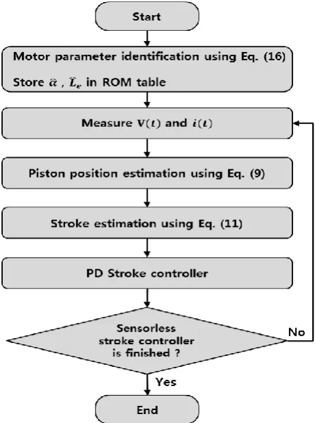
[image:4.595.316.546.381.690.2]

Fig. 3 shows a flow chart for the closed-loop sensorless stroke control using the motor parameters identification method I (PIM I). First, a linear variable differential transformer (LVDT) is installed on the liner motor to measure the piston position. Then, a closed-loop stroke control system is implemented, and ( ), ( ), and ( ) = 1, 2, … are measured in the steady state. Using these measured state variables, the identified motor parameters ̂ and ̂ are obtained using Eq. (16) and stored in the ROM table. Next, the sensorless stroke control loop is executed repeatedly.

(5)

International Journal of Emerging Technology and Advanced Engineering

[image:5.595.334.524.148.301.2]

261 The experimental apparatus of a sensorless stroke controller for linear compressors has been implemented as shown in Fig. 4. The CPU chip is a TMS320C2000 (Texas Instruments, USA). For experimental study, a 2.2 kW linear compressor is chosen as shown in Table 1. The set-point value of the stroke is 0.02 m. The running frequency is set to 60 Hz.

Fig. 4. Implemented experimental apparatus.

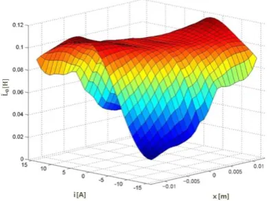
The identified motor parameters ̂ and ̂ obtained using Eq. (16) are shown in Figs. 5 and 6, respectively. As can be seen from Fig. 5, ̂ is approximately 30–55 N/A for the piston position in the range of −0.01 m < ( ) < 0.01 m, and the current is in the range of −10 A < ( ) < 10 A. However, one can observe from Fig. 6 that ̂ is approximately 0.03–0.12 H for the same range of the piston position and the current.

Table 1. Linear motor specifications.

Rated output power Rated voltage Rated current Rated stroke Resonant frequency

𝑅𝑒

𝐿𝑒

2.2 kW 220 Vrms 7 Arms 0.02 m

[image:5.595.80.249.215.352.2]

60 Hz 2.5 Ω 55 N/A 0.12 H

Fig. 5. Three-dimensional plot of the identified force constant ̂.

Up to now, it has been found to be costly and difficult to install a piston position sensor for measuring the stroke. It has also been found that piston position estimation requires information of the motor parameters which are not constant and vary as functions of the piston position and the motor current. Therefore, the motor parameters 𝛼 and 𝐿𝑒, which have substantial influence on the dynamic performance of the closed-loop stroke control system, should be identified as functions of piston position and motor current, stored in ROM table, and used for accurate estimation of piston position. However, PIM I has the demerit of demanding a large memory space for storing the identified motor parameters. Therefore, in this study, another technique is proposed for solving this problem.

[image:5.595.53.288.467.601.2] [image:5.595.331.526.503.650.2]

(6)

International Journal of Emerging Technology and Advanced Engineering

262 IV. MOTOR PARAMETERS IDENTIFICATION METHOD II

As an approach for reducing the amount of identified motor parameter data, the identified force constant ̂ shown in Fig. 5 is approximated to be the following second-order surface:

( , , ) = 02+ 1 2+ 2 + 3 + 4 + 5 (17)

Where is the current, is the piston position, and is the function representing the approximated force constant. Here, let data sets of the identified force constant be { ( ₀, ₀, ₀) , ( ₁, ₁, ₁) , … ( −1, −1, −1)}. Then, one obtains

[ 0 1 ⋮ −1

] = [

0 2

02 0 0 0 0 1

1 2

12 1 1 1 1 1

⋮ ⋮ ⋮ ⋮ ⋮ ⋮

−1 2

−12 −1 −1 −1 −1 1]

[ 0 1 2 3 4 5]

(18)

From this, one can obtain

[

0 1 2 3 4 5]

= 𝑑

[

0 2

0 0 0 0 1 1

2 1 2

1 1 1 1 1

⋮ ⋮ ⋮ ⋮ ⋮ ⋮

−1 2

−12 −1 −1 −1 −1 1]

[

0 1

⋮

−1

] (19)

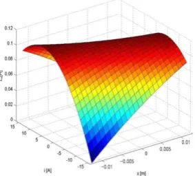
Using data sets of the identified force constant ̂ given in Fig. 5, Eq. (19) is solved, and the second-order approximation of ̂, shown in Fig. 7, is finally obtained. Similarly, the identified inductance ̂ shown in Fig. 6 can also be approximated to the second-order surface: ( , , 𝐿) 𝐿 = 02+ 1 2+ 2 + 3 + 4 + 5 (20)

[image:6.595.350.509.147.279.2]

Using the similar procedure as Eqs. (17–19), we can obtain ( = ,1, ,5) and the result shown in Fig. 8.

Fig. 7. Second-order approximation of ̂.

[image:6.595.48.280.223.427.2]

Fig. 9 shows a flow chart for the closed-loop sensorless stroke control using the motor parameters identification method II (PIM II). At first, the identified motor parameters ̂ and ̂ are obtained using Eq. (16) by the same procedure as in PIM I. Next, the second-order approximations of ̂ and ̂ are made using Eq. (19), and , ( = ,1, ,5) are stored in a ROM table. Finally, the sensorless stroke control loop is executed repeatedly. Here, one should note that and are to be calculated using Eqs. (17) and (20) for every execution of the sensorless stroke control loop.

[image:6.595.359.501.452.580.2]

(7)

International Journal of Emerging Technology and Advanced Engineering

[image:7.595.47.280.132.492.2]

263 Fig. 9. Flow chart for the stroke control using PIM II.

[image:7.595.334.527.132.277.2]

V. MOTOR PARAMETERS IDENTIFICATION METHOD III Next, in order to decrease the identification errors of PIM II, the identified motor parameters are divided into 4 parts and are approximated individually as shown in Fig. 10. The identified inductance ̂ is composed of the 4 surfaces, 1, 2, 3, and 4, expressed in the form of Eq. (20).

Fig. 10. Division into 4 parts and approximation of ̂.

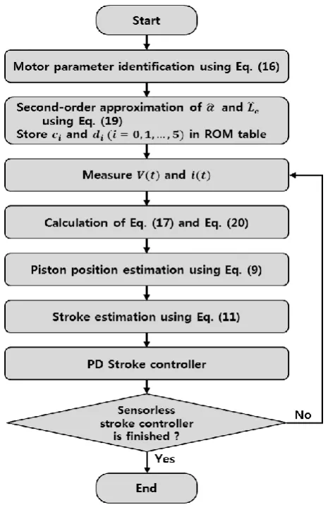
Fig. 11 shows a flow chart for the closed-loop sensorless stroke control using the motor parameters identification method III (PIM III). At first, the identified motor parameters ̂ and ̂ are obtained using Eq. (16) by the same procedure as PIM II. Next, for each surface ( = 1,2,3,4), the second-order approximations of ̂ and ̂ are made using Eq. (19), and , ( = ,1, ,5) are stored in a ROM table. Finally, the sensorless stroke control loop is executed repeatedly. Note also that and are to be calculated using Eqs. (17) and (20) for every execution of sensorless stroke control loop as in PIM II.

VI. EXPERIMENTS AND DISCUSSIONS

(8)

International Journal of Emerging Technology and Advanced Engineering

[image:8.595.51.275.101.579.2]

264 Fig. 11. Flow chart for the stroke control using PIM III.

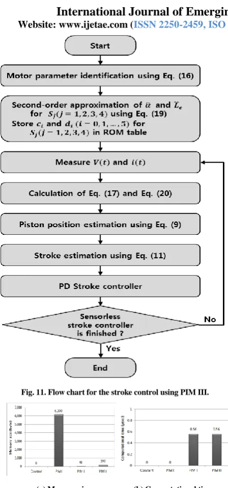
(a) Memory size (b) Computational time

Fig. 12. Memory size and Computional time using PIM III.

Fig. 12. (a) Memory size needed for storage and (b) computational time needed for the calculation of ̂ and ̂ .

First, the memory size that is needed for storing the identified motor parameters ̂ and ̂ in a ROM table is compared. If they are set to be constant, the memory size of 8 bytes is needed. As shown in Fig. 12 (a), PIM I, PIM II, and PIM III need memory sizes of 6,200 bytes, 48 bytes, and 192 bytes, respectively.

Second, the computational time needed for calculating and in every execution of sensorless stroke control loop is compared. The methods Constant and PIM I do not require calculation using Eqs. (17) and (20), which makes their computational times zero. However, PIM II and PIM III require a computational time of 0.56 μs to calculate Eqs. (17) and (20). Fig. 12 (b) shows the computational time needed for the calculation of and in every execution of sensorless stroke control loop.

[image:8.595.318.553.391.532.2]

Finally, the stroke control error is compared. In the closed-loop sensorless stroke control system shown in Fig. 2, the stroke command is set to be 0.011 m. In the steady state, we obtained stroke errors of 5.2%, 1.7%. 2.9%, and 2.6%, for Constant, PIM I, PIM II, and PIM III, respectively. We did a similar experimental study while the stroke command was increased from 0.011 to 0.019 m. Fig. 13 shows the experimental results of the stroke control error versus stroke command. In this experiment, we can see that the average values of stroke error were 6.36%, 1.74%, 2.88%, and 2.66%, for Constant, PIM I, PIM II, and PIM III, respectively.

Fig. 13. Stroke control error versus stroke command.

VII. CONCLUSION

In this paper, a closed-loop sensorless stroke control system for a linear compressor has been designed. The motor parameters are identified as functions of the piston position and motor current. Then, they are stored in a ROM table and used later for accurate estimation of piston position. The performances of the various motor parameter identification algorithms are evaluated by experimental studies.

(9)

International Journal of Emerging Technology and Advanced Engineering

265 However, PIM I has the demerit of demanding a large memory space for storing the identified motor parameters. In order to decrease the memory size, PIM II or PIM III may be chosen for the motor parameter identification algorithm if the additional computational time needed for the calculation of and 𝐿 in every execution of sensorless stroke control loop is negligible.

Acknowledgement

This research was supported by Basic Science Research Program through the National Research Foundation of Korea(NRF) funded by the Ministry of Education, Science and Technology(No.2011-0023587)

REFERENCES

[1] Reuven Unger, ―Linear compressors for non-CFC refrigeration,‖ Proceedings International Appliance Technical Conference, pp.373-380, May, 1996.

[2] Robert Redlich, Reuven Unger, Nicholas van der Walt, ―Linear compressors : motor configuration, modulation and systems,‖ Proceedings International Compressor Engineering Conference, pp.68-74, July, 1996.

[3] Reuven Unger, ―Linear compressors for clean and specialty gases,‖ Proceedings International Compressor Engineering Conference, pp.73-78, July, 1998.

[4] Reuven Unger, ―Development and testing of a linear compressor sized for the european market,‖ Proceedings International Appliance Technical Conference, pp.74–79, May, 1999. [5] Masayuki Sanada, Shigeo Morimoto, and Yoji Takeda, ―Analyses

for sensorless linear compressor using linear pulse motor,‖ Proceedings Industry Applications Conference, pp. 2298–2304, Oct., 1999.

[6] Yee-Pien Yang and Wei-Ting Chen, ―Dual stroke and phase control and system identification of linear compressor of a split-stirling cryocooler,‖ Proceedings Decision and Control, pp.5120–5124, Dec., 1999.

[7] Gye-young Song, Hyeong-kook Lee, Jae-yoo Yoo, Jin-koo Park, and Young-ho Sung, ―Development of the linear compressor for a household refrigerator,‖ Proceedings Appliance Manufacturer Conference & Expo, pp.31-38, Sept., 2000.

[8] Hyuk Lee, Sunghyun Ki, Sangsub Jung, and Won-hag Rhee, ―The innovative green technology for refrigerators - Development of Innovative linear compressor-,‖ International Compressor Engineering Conference at Purdue, pp.1419-1424, July, 2008. [9] B. J. Huang and Y. C. Chen, ―System dynamics and control of a

linear compressor for stroke and frequency adjustment,‖ Journal of Dynamic Systems, Measurement, and Control , Vol.124, pp.176-182, March, 2002.

[10] Kyeong-bae Park, Eun-pyo Hong, Ki-chul Choi, and Won-hyun, Jung, ―Linear compressor without position controller,‖ International Compressor Engineering Conference at Purdue, pp.C119-C125, July, 2004.

[11] N. Chen, Y. J. Tang, Y. N. Wu, X. Chen, and L. Xu, ―Study on static and dynamic characteristics of moving magnet linear compressors,‖ Cryogenics, vol.47, pp.457–467, 2007.

[12] Tae-Won Chun, Jung-Ryol Ahn, Hong-Hee Lee, Heung-Gun Kim, and Eui-Cheol Nho, ―A novel strategy of efficiency control for a Linear compressor system driven by a PWM inverter,‖ IEEE Trans. on Industrial Electronics, Vol.55, No.1, pp.296-301, Jan., 2008.

[13] Jinquan Zhang, Yunfeng Chang, and Ziwen Xing, ―Study on self-sensor of linear moving magnet compressor’s piston stroke,‖ IEEE Sensors Journal, Vol.9, No.2, pp.154-158, Feb., 2009. [14] Gyu-Sik Kim, ―Sensorless control for linear compressors,‖ The

Trans. of The Korean Institute of Power Electronics, Vol.10, No.5, pp.421-427, Oct., 2005.