MODIFICATION OF NEURAL NETWORK ALGORITHM USING CONJUGATE GRADIENT WITH ADDITION OF WEIGHT INITIALIZATION

OBJECT LOCALIZATION AND PATH OPTIMIZATION

USING PARTICLE SWARM AND ANT COLONY

OPTIMIZATION FOR MOBILE RFID READER

1

MOHD ZAKI ZAKARIA , 2MD YUSOFF JAMALUDDIN

1

Faculty of Computer and Mathematic, University Technology MARA, Shah Alam Malaysia

2_{Department of Electrical, Electronic and System Engineering, Universiti Kebangsaan Malaysia}

E-mail: [email protected] , [email protected]

ABSTRACT

Optimization for an RFID reader is an important technique to reduce the cost of hardware; we need to define the location of the RFID reader to ensure the node will be fully covered by the reader. It is also essential to find the best way to place the nodes in a given area that guarantees 100% coverage with least possible number of readers. In this paper, we propose a novel algorithm using particle swarm and ant colony optimization techniques to achieve the shortest path for an RFID mobile reader, and at the same time, ensure 100% coverage in the given area. For path optimization, the mobile reader traverses from one node to the next, moving around encountered obstacles in its path. The tag reading process is iterative, in which the reader arrives at its start point at the end of each round. Based on the shortest path, we use an algorithm that computes the location of items in the given area. After development of a simulation prototype, the algorithm achieves promising results. Experimental results with benchmarks having up to 150 nodes show that the ant colony optimization (ACO) method works more effectively and efficiently than particle swarm optimization (PSO) when solving shortest path problems.

Keywords: RFID, Path Optimization, PSO, ACO

1. INTRODUCTION

In recent years, Radio Frequency Identification (RFID) technology has become popular in many industries, including manufacturing, automotive services and social retailing. In other words, this technology has had a significant influence on society lifestyle. With the ubiquity of RFID deployment, there is a need to ensure that any object can be traced easily when it is tagged. This is accomplished with RFID technology, together with a wide variety of objects. Generally, RFID is able to tag, trace and check an object, and RFID tags are attached to objects. Tags contain important information about an object, such as its unique ID number, manufacture date and product composition.

RFID technology uses radio waves to enable the communication between readers and tags. The RFID tag is a device that stores an object’s data such as its ID, and transmits it to the reader in a contactless manner using radio waves. Objects are identified when a tag transmits this

information back to the readers within the interrogation range. The reader is a device that can read data from and write data to compatible RFID tags. RFID readers can be fixed (static), or mobile (within a predefined physical area). Objects are identified when tags transmit this information back to the readers within the interrogation range.

Tags can be classified in two main types, i.e., passive and active. Most of applications use passive tags because they are cheaper and have a smaller size compared to active tags. A passive tag reader can detect objects distanced up to eight meters in the UHF band [1]. .In order to provide complete coverage for a given area, RFID readers must be arranged in an efficient manner, in order to reduce hardware (RFID reader) costs as much as possible.

Optimization (PSO) and Ant Colony Optimization (ACO) techniques that incorporate the nearest neighbor for the movement of RFID mobile readers. The optimum path (i.e., shortest path) information obtained is used to compute the location of objects within the given area using the triangulation technique.

We aim to find the best method to place the RFID readers (nodes) in a given area in order to guarantee 100% coverage with a minimum number of readers. In the first phase we develop a prototype of the software simulation to determine how many RFID fixed readers are required to cover a given area based on hexagonal packing, which produces approximately 90% efficiency, as depicted in Figure 1. Every hexagon is equivalent to one RFID reader [2]. The coverage of a wireless sensor network may be approximated by a disk of a prescribed radius (sensing range). Coverage can be computed by taking the union of individual coverage areas of all sensors (readers) in the network. This can be performed by assuming that each circle is a hexagon which attaches with another (Fig. 1). We assume all the readers have the same sensing and transmission range.

In the second phase, the location of the RFID reader that we calculated previously is used as a reference point the mobile reader visits in a certain period of time. We proposed to use the mobile RFID reader to reduce hardware (reader) costs, and eliminate readers’ interference. The mobile reader is moved from one point (node) to another point based on the shortest path computed using PSO and ACO for the given dimension area. The tag reading process by the mobile RFID reader is repeated when the reader arrives to its start node in the loop. This process repeated in an iterative fashion.

In the third phase, we start the algorithm with an initialization process to determine the number of tags to be used in the given area. The process continues by placing tags at random in the same area. The process continues which tags detecting by mobile RFID reader 3 times at different location or point in the given dimension area) we continue the process by detecting a reader and it is done until all three readers are detected the tags. Then we continue with the calculation to determine the position of tags by using the equations discussed in Section 3. The equation is based on the data of the received signal strength indication (RSSI) that is obtained during the detection process.

There are four main contributions in this paper. First, the algorithm can be used to eliminate redundant sensors or readers without affecting network coverage, so that the mobile RFID reader a less amount of nodes. Second, an algorithm for the RFID mobile reader for path optimization using PSO and ACO techniques incorporating the nearest neighbour is presented. Third, the algorithm determines the location of object/tags in that area covered by the mobile RFID reader. Finally, the design of the algorithm is able work with any design area, whether it is asymmetrical or symmetrical. In addition, the algorithm has the ability to define the position of the obstacles based on a real working environment.

This paper is organized as follows. Section 2 presents the related work in this area. Section 3 discusses object localization. Section 4 presents the proposed algorithm. Section 5 presents the algorithm simulation and results, while Section 6 discusses the results of the simulation. Finally, Section 7 gives a conclusion and recommendations for future work.

2. RELATED WORK

Global Positioning Systems (GPSs) widely uses outdoor localization models that rely on satellites to determine an object’s location. GPS is not suitable for tracking indoor localization because of high costs, high power consumption, and limited power tag’s object (P. Enge 1999). In order to overcome the disadvantage of GPS and effectively track objects in indoor environments, researchers developed several techniques and algorithms, including scene analysis, proximity or triangulation. Location Identification based on Dynamic Active RFID Calibration (LANDMARC) uses the conception of a reference tag, which is the tag fixed in the known location (Ni, L.M et al 2003). The system provides a signal strength for comparison with the signal strength of the object tag. Due to a reference tag being near an object tag, it suffers similar effects around the environment. The Landmarc approach requires signal strength information from each tag to readers, if it is within the detectable range. For three dimension (3D) location sensing based on radio signal strength, the SpotON algorithm was developed, which is a coordination and aggregation algorithm used to measure the tag location based on signal strength (Hightower &Borriello 2000).

corresponds to a reference tag. Huang et al. (2006) proposed probabilistic localization techniques to detect the object using three steps. First, the propagation variables are calibrated using on-site reference tags, and then the distance between the object (targeted tag) and the readers is estimated with a probabilistic RSS model. Finally, the location of the tag is determined by applying a Bayesian inference technique.

RFID technology has also been used to guide blind people to find the shortest route from their current location to a destination. This technology also helps them when they get lost by automatically detecting the route, and recalculating a new route to the same destination [3]. The system embeds RFID tags into a footpath that can be read by an RFID reader with a cane antenna. The system is also used for navigation in rescue operations involving hazardous environments, where it is difficult to find an emergency exit. The indoor guidance system [4] uses RFID technology to find a guidance path for important places, such as museums, hospitals, airport terminals and exhibition halls.

The most challenging task is to achieve the shortest path for a network by minimizing the cost (distance) inside a given area. The shortest path has been used extensively for other purposes, such as vehicle routing in the transportation system [5], path planning in robotics [6] and traffic routing in communication networks [7]. S. Anusha proposed an application for complete coverage within a predefined period of time using mobile RFID readers in a symmetrical area [8]. The system proposed by S. Anusha only catered for symmetrical area, and within the area covered by RFID mobile readers, she assumes the areas only locate the proper stacked shelves. The given area is divided into many sectors, and each sector is catered by one mobile reader. The path shown in Anusha’s work (i.e., zig zag type) is similar for every sector. Ammar et al. presents the investigation of PSO to solve the shortest path routing problem using a modified priority based indirect encoding, incorporating a heuristic operator for reducing the possibility of loop formation in the path construction process [9].

3. OBJECT LOCALIZATION

Many research works have proposed algorithms for localization and positioning applications of RFID readers and tags (P. Bahl & V. N. Padmanabhan 2000) (D. Nicules&B.Nath

2003) (Savvides & Han 2001). In general, one of the most fundamental issues in wireless sensor networks is reader coverage, in which every point of the selected area must be within the sensing range of at least one sensor network. In the literature, this problem has been proposed in many different ways, for example, using mobile readers (Savvides & Strivastava 2001). The coverage of a wireless sensor network may be approximated by a disk of a prescribed radius (sensing range). Coverage can be computed by taking the union of individual coverage areas of all sensors (readers) in the network.

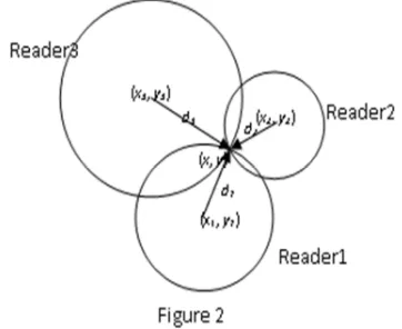
Figure 2 illustrates a system model for a tracking object. The circles represent the coverage for three RFID readers. The estimated position is determined using received signal strength indicator (RSSI) mapping to an approximate distance d1, d2 and d3 respectively. Location for reader1 is at coordinate (x1, y1), reader2 at (x2, y2) and reader 3 at (x3, y3) respectively.

We are able to calculate the position of an object based on the following equations:

where x1 and y2 is the location of reader 1; x2 and y2

is the location of reader 2; x3 and y3 is the location

of reader 3; d1 is the distance targeted tag (object)

and reader 1; d2 is the distance targeted tag (object)

and reader 2; and d3 is the distance targeted tag

follows:

We can replace these by:

Hence, the location of the targeted tag (object) is given by:

1 2

| | | |

4. PROPOSED ALGORITHM

The main objective of path optimization is to find the proper variables which yield the minimum or maximum objective function value under constrained conditions. In this section, we developed a simulation program using PSO and ACO techniques to achieve the optimized path of RFID mobile readers, in which both techniques incorporate the nearest neighbor.

A. Particle Swarm Optimization

Particle swarm optimization (PSO) is a population-based stochastic optimization technique that originates from nature and evolutionary computations, developed by Kennedy and Eberhart (10). This method finds an optimal solution within a population (i.e., a swarm). The PSO algorithm flow consists of a population of individuals referred to as “particles”. Every particle is a potential solution to an n-dimensional problem. The group can achieve the solution effectively by using common information shared by the group, and the information is owned by the particle itself. The particles change their state by “flying” around in an n-dimensional search space based on the

velocity, updated until a relatively unchanging state has been encountered, or until computational limitations are exceeded. PSO contains two types of learning: cognitive and social learning.

PSO has been successfully applied to solve many optimization problems, and has attracted great attention in power system design, data classification, pattern recognition and image processing, robotic applications, decision making for the stock market, and simulation and identification of emergent systems. With reference to the original PSO, each particle knows its best value so far (pbest), velocity, and position. Additionally, each particle knows the best value in its neighbourhood (gbest). A particle modifies its position based on its current velocity and position.

For all iterations, any particle is updated by following two "best" values. The first one is the best solution (fitness) it has achieved so far, referred to as pbest, and the fitness value is also stored. Another "best" value that is tracked by the particle swarm optimizer is the best value obtained so far by any particle in the population, which is called global best (gbest).

The velocity vector update equation which controls the direction the particle will move in the design space is calculated using:

! "

# # $ (1)

where is the velocity vector, is a modified velocity vector and is a positioning vectorof particle i at generation k. Also, is the best position found by particle i and $ is the best position found by the particle’s neighbourhood of the entire swarm; and _# are the cognitive and social coefficients which are used to bias the search of a particle toward its individual’s own best history (pbest), and the best history accumulated by sharing information among all particles of the entire swarm (gbest). ω is the inertia weight factor to control the level of contribution from the particle’s current velocity vector to the new velocity factor. Large values of ω facilitate exploration and searching new areas, while small values of ω navigate the particles to a more refined search. The velocity equation includes two different random parameters, represented by a variable and _# to ensure good exploration of the search space and avoid entrapment in local optima. The direction and velocity of the particle is based on its current velocity vector, previous best location (pbest) and global best location (gbest).

RFID reader. Hence, the particle swarm attempts to find the optimal path for the mobile RFID reader to move from one node to another. This technique randomly generates a population of particles within the given dimension area. Therefore, the swarm attempts to find the optimal path that will be used for the mobile RFID reader to move to every single node in the given area.

The PSO algorithm is the equation of the sigmoid function for the updating velocity:

6$ 7

7 89:;<=>

The modified position vector is obtained using:

? 1 6@ A B 6$ C "

0 otherwise

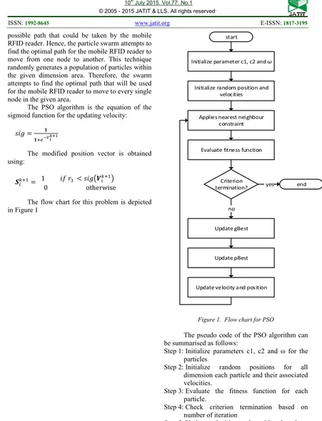
The flow chart for this problem is depicted in Figure 1

start

Initialize parameter c1, c2 and ω

Initialize random position and velocities

Applies nearest neighbour constraint

Evaluate fitness function

Criterion

termination? yes end

no

Update gBest

Update velocity and position Update pBest

Figure 1. Flow chart for PSO

The pseudo code of the PSO algorithm can be summarised as follows:

Step 1: Initialize parameters c1, c2 and ω for the particles

Step 2: Initialize random positions for all dimension each particle and their associated velocities.

Step 3: Evaluate the fitness function for each particle.

Step 4: Check criterion termination based on number of iteration

Step 5: Update velocities and position based on nearest neighbour constraint.

Step 6: Update local best (pbest), which compares the current value of fitness function with the previous best value of the particles.

the particles.

Step 8: Apply state transition based on nearest neighbour constrain and the process will continue till end condition when maximum number of iterations is reached

B. Ant Colony Optimization

The ant colony optimization (ACO) is a meta-heuristic optimization technique for hard combinatorial optimization problems. We examine the ant colony system (ACS) as a representative of the ACO technique. The ACS has three main aspects: i) the state transition rule provides a direct way to balance between exploration of new edges and exploitation of a priori and accumulated knowledge about the problem; ii) the global updating is applied only to edges which belong to the best ant tour; and iii) while ants construct a solution, a local pheromone updating rules applied.

Basically, for the ACS process, F ants are initially put on G nodes chosen according to some initialization rule (e.g., randomly). Each ant builds a path by repeatedly applying the state transition rule. During constructing its path, an ant make some changes to the amount of pheromones on the visited edges by applying the local updating rule. Once all ants have finished their path, the amount of pheromones on edges is modified again by applying the global updating rule. The path with a high amount of pheromones is preferred by the ants, hence, they will choose the short path.

a. State transition rule

The ACS transition rule, also referred to as

the pseudo-random-proportional rule, was

developed to explicitly balance the exploration and exploitation abilities of the algorithm. In ACS, the probability for an ant to move from node r to node

s depends on a random variable q and q0, as shown

below:

[

] [

]

{

}

( () 0

ACS q q if S u r u r s r

p u J r

k k ≤     ⋅ = ∈ β η τ

Where q is a uniformly distributed random variable [0, 1], q0 is between 0 and 1, and S is a

variable which selected according to the probability distribution.

Jk(r) is the set of feasible components; that

is, edges (r, s), where r is the current node and s is a next node which is not yet visited by the k-th ant.

(r, u) are the other edges, where u is all nodes not yet visited by the k-th ant. The parameter β (β ≥ 0) controls the relative importance of the pheromones versus the heuristic information η(r, s), which is given by: , 1 ) , ( rs d s r = η

where in the mobile RFID reader, drs is the distance

between nodes r and s, and τ(r, s) is the pheromone trails which refer to desirability of visiting node s

directly after r. For implementation purposes, the pheromone trails are collected into a pheromone matrix, whose elements are the all of τ(r, s).

b. Global updating rule

The global pheromone update is applied at the end of each iteration to one ant, which can be either the iteration-best ant or the best-so-far ant. The pheromone updating rules are designed so that they tend to give more pheromone to edges which should be visited by ants.

c. Local pheromone updating rule

The local pheromone update is performed by all ants after each construction step using:

0 1 (1 ) ( , )

) ,

( ζ τ τ

τ r s t₊ = − ⋅ r s t +

where ζ ∈[0, 1] is the pheromone decay coefficient, and τ0 is the initial value of the pheromone.

The main goal of the local update is to diversify the search by decreasing the pheromone concentration on the traversed edges. Thus, the ant would choose another route to produce different solutions. This would prevent several ants to produce identical solutions during an iteration.

start

Initialize parameter t, α, ρ and q0

Calculate τ0

Applies local pheromone updating

Evaluate fitness function

Criterion

termination? yes end

no

Applies global pheromone updating Pheromone Initialize

Applies state transition rule based on nearest neighbour

constraint

Figure 2.Figure 2. Flow chart for ACO

The pseudo code of the ACO is as follows: Step 1: Initialize parameter t, α, ρ, q0, nk, and

calculate τo

Step 2: For every link (r,s), perform the pheromone initialization τ (r,s) = τo;

Step 3: Initialize number of iterations and apply state transition rule based on neighbour constraint

Step 4: Apply local pheromone update until all ants have built a complete solution

Step 5: Calculate fitness

Step 6: Check criterion termination based on number of iteration.

Step 7: Apply global pheromone updating for the best solution produced by ants

Step 8: Apply state transition based on nearest neighbour constrain and the process will continue till end condition when maximum number of iterations is reached.

5. ALGORITHM SIMULATION AND

RESULTS

A. Simulation Setup

Numerous research activities have been proposed in localization and positioning applications of RFID readers and tags [15]. In general, one of the most fundamental issues in wireless sensor networks is reader coverage. Every point of the selected area must be within the sensing range of at least one sensor network. In the literature, solutions to this problem have been proposed in many different ways, e.g., using a mobile reader [16]. The coverage of a wireless sensor network may be approximated by a disk of a prescribed radius (sensing range). Coverage can be computed by taking the union of individual coverage areas of all sensors (readers) in the network. This can be done by assuming that each circle is a hexagon which attaches with another, as shown in Figure 1.

In this experiment, the number of nodes depends on the dimension of the area and interrogation range that we set for the mobile RFID reader. If the dimension of area is large then the number of nodes that a mobile RFID reader traverses is increased. In other words, the interrogation range influences the number of nodes the mobile RFID reader visits.

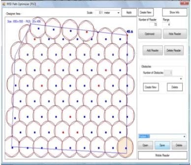
Figure 3.Figure 1: A typical 76 nodes (number of nodes that mobile RFID reader visits) with an interrogation

interrogation of a reader. To address this problem, the software simulation that is developed can define the read range of the RFID reader and obstacles inside the area covered, based on user requirement. In Figure 1, the RFID mobile reader skips the red points (nodes) because obstacles are positioned on these points. The system prototype we develop determines the coordinate of each reader in an area to optimize the reader usage and its coverage.

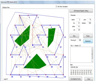
Figure 4.Figure 2: A typical 36 nodes (RFID reader) with an interrogation range of 5 meters, and 3 obstacles

in the given area using PSO

Figure 5.Figure 3: A typical 36 nodes (RFID reader) with an interrogation range of 5 meters, and 3 obstacles

in a given area using ACO

In this experiment, we start the algorithm with an initialization process to determine the number of readers to be used in a given area, and the system optimizes the number of readers based

on the area. Using PSO and ACO techniques, the RFID mobile reader scans every single node inside the area, as shown in Figures 2 and 3 above. PSO and ACO attempt to find a path to complete a circle, in which the minimum path (distance) is chosen as the optimal path. We run every algorithm successively for 100 and 500 iterations under the same initialization conditions, then record the minimum and maximum paths for PSO and ACO. Figures 2 and 3 show the number of readers for a given area (which have 3 obstacles that the mobile reader cannot move through) for PSO and ACO respectively. The mobile RFID reader can start at any node at random.

6. RESULT AND DISCUSSION

We used the following configuration for the PSO and ACO algorithm. For the PSO algorithm, the number of particle is 10, the cognition factor c1

and social factor c2 are 1.4, and the inertia weight w

is 0.4 to 0.9. Whereas for the ACO algorithm, the population (i.e., number of ants) is 10, ρ and ζ are 0.1, β is 2 and q0 is 0.9. All the algorithms were run

Table 1: The result of optimization path using PSO and ACO for 150 nodes and 5 obstacles

Method PSO ACO

# Running 100 500 100 500 100 500 100 500

# iteration 100 100 500 500 100 100 500 500

Max path 7938.29 7956.39 7533.10 753.57 6999.93 6966.88 6509.91 6313.98 Min Path 4721.24 4611.82 4700.21 4661.82 4611.82 4611.82 4661.82 4661.82 Avg Path 5831.56 5861.89 5524.71 5521.39 5613.05 5543.36 5424.99 5221.39

Std Dev 331.66 320.77 280.78 251.30 318.23 311.12 268.80 219.46

Table 2: The percentage of optimization path using PSO for 150 nodes and 5 obstacles

Method PSO

# Running 100 ₅₀₀ 100 ₅₀₀

# Iteration 100 100 500 500

% % % %

Uncompleted 5552 55.52% 26781 53.56% 26131 52.26% 120023 48.01%

Completed FALSE 2401 24.01% 12921 25.84% 13393 26.79% 60283 24.11%

TRUE 2047 20.47% 10298 20.60% 10476 20.95% 69694 27.88%

Total 10000 100.00% 50000 100.00% 50000 100.00% 250000 100.00%

Max Conv at # 100 100% 100 100% 489 98% 491 98%

Min Conv at # 60 60% 60 60% 125 25% 147 29%

Avg Conv 90.21 90.21% 82.32 82.32% 345.32 69.06% 320.26 64.05%

Std Dev Conv 15.41 15.34 250.77 250.45

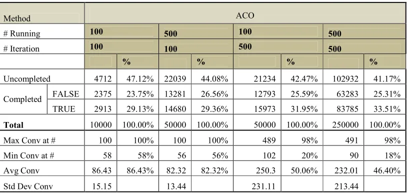
Table 3: The percentage of optimization path using ACO for 150 nodes and 5 obstacles

Method ACO

# Running 100 500 100 500

# Iteration 100 100 500 500

% % % %

Uncompleted 4712 47.12% 22039 44.08% 21234 42.47% 102932 41.17%

Completed FALSE 2375 23.75% 13281 26.56% 12793 25.59% 63283 25.31%

TRUE 2913 29.13% 14680 29.36% 15973 31.95% 83785 33.51%

Total 10000 100.00% 50000 100.00% 50000 100.00% 250000 100.00%

Max Conv at # 100 100% 100 100% 489 98% 491 98%

Min Conv at # 58 58% 56 56% 102 20% 90 18%

Avg Conv 86.43 86.43% 82.32 82.32% 250.3 50.06% 232.01 46.40%

the ACO algorithm significantly outperformed the PSO algorithm. This demonstrates that the ACO algorithm has faster convergence and adaptability. Simulation results show that for the ACO algorithm, the minimum path (best value) is 4611.82 for 100 runs (and 100 iterations for each run). The completed and true path for ACO is higher than the PSO. The standard deviation value for the ACO is better than that of the PSO at iteration 100.

7. CONCLUSION

In this experiment, we proposed a novel algorithm for an RFID mobile reader to optimize the path and cover a given area using PSO and ACO techniques. Both techniques we incorporate with nearest neighbor to achieve better results. After development of a simulation prototype, and evaluative experimentation of the prototype, the feasibility and effectiveness of the ACO algorithm significantly outperform the PSO algorithm. The results show that the ACO algorithm achieve promising results, and has competitive potential for solving discrete optimization problems like path optimization compared to the PSO algorithm.

As recommendation for future work, it would be worthy to further investigate whether the use of both the PSO and ACO algorithms in combination would achieve better accuracy. We plan to further investigate the functionality of this combination approach and present our experimental results in a subsequent paper.

REFERENCES

[1]. Finkenzeller, K. : RFID Handbook, 2003. Fundamental and applications in contactless

smart cards and

identificationdritteedn.Chichester : John Wiley.

[2]. http://en.wikipedia.org/wiki/Packing_proble m#Circles_in_square

[3]. SakmongkonChumkamon, PeranittiTuvaphanthaphiphat,

PhongsakKeeratiwintakorn, Proceedings of ECTI-CON 2008

[4]. Chou L.D., Wu C.H., Ho S.P., Lee C.C. and Chen J.M. (2004) Requirement Analysis andImplementation of Palm-based MultimediaMuseum Guide Systems. IEEE 18th International

[5]. F.B. Zahn, C.E. Noon, Shortest path algorithms: An evaluation using real road networks, Transport. Sci. 32 (1998) 65–73. [6]. G. Desaulniers, F. Soumis, An efficient

algorithm to find a shortest path for a car-like robot, IEEE Trans. Robot.Automat. 11 (6) (1995) 819–828.

[7]. Moy, J., 1994. Open Shortest Path First Version 2. RFQ 1583, Internet Engineering Task Force. http://www.ietf.org.

[8]. S. Anusha& Sridhar Iyer, 2005. A Coverage Planning Tool for RFID Networks With Mobile Readers: EUC workshops, LNCS 3823

[9]. AmmarW.Mohemmed et al. Solving shortest path problem using particle swarm optimization. Applied Soft Computing 8(2008) 1643-1653

[10]. J. Kennedy, R.C. Eberhart, Particle swarm optimization, in: Proceedings of the IEEE International Conference on Neural Networks, 1995, pp.1942–1948.

[11]. [11] Goldberg, D.E., 1989. Genetic Algorithms in Search, Optimization and Machine Learning.Addison-Wesley, Reading, MA.

[12]. Starkweather, T., Whitley, D., Whitley, C., Mathial, K., 1991. A comparison of genetic sequencing operators. In: Proceedings of the Fourth International Conference on Genetic Algorithms, Los Altos, CA, pp. 69–76. [13]. Oliver, I., Smith, D., Holland, J., 1987. A

study of permutation crossover operators on the traveling salesman problem. In: Proceedings of the Second International Conference on Genetic Algorithms, London, pp. 224–230.

[14]. Knosala, R., Wal, T., 2001. A production scheduling problem using genetic algorithm.Journal of Materials Processing Technology 109 (1–2), 90–95.

[15]. P.Bahl& V.N. Padmanabhan, 2000. RADAR: an in-building RF-based user location and tracking systems, in IEEE INFOCOM, pg775-784