February 19, 1998
Smooth Scheduling in a Cell-Based
Switching Network
Thomas L. Rodeheffer
and
James B. Saxe
Systems Research Center
130 Lytton Avenue Palo Alto, CA 94301
http://www.research.digital.com/SRC/
Smooth Scheduling in a Cell-Based
Switching Network
Thomas L. Rodeheffer and James B. Saxe
© Digital Equipment Corporation 1998
Abstract
Contents
1. Introduction... 1
2. Background ... 1
3. The basic recursively balanced scheduling method... 5
3.1. Recursive splitting of the scheduling frame ... 6
3.2. The splitting step ... 7
3.3. An example of the splitting step... 9
4. Degree of smoothness achieved by the basic method... 12
4.1. Maximum scheduling discrepancy in a given schedule ... 14
4.2. Maximum scheduling discrepancy in legal schedules... 16
4.3. A bound for msd in recursively balanced schedules ... 16
4.4. Actual msd values for certain loads ... 19
5. Output link smoothness ... 21
6. Odd-size frames ... 23
7. Implementation ... 24
7.1. Hardware description ... 24
7.2. Software environment ... 25
7.3. Implementation overview... 26
7.4. Implementation details ... 28
7.5. Slot extraction algorithm... 29
7.6. Performance ... 31
7.7. An additional constraint ... 33
8. Potential improvements ... 33
8.1. Parallelism... 33
8.2. Aggregating flows ... 34
8.3. Shift in strategy for small subframes... 34
9. Conclusions... 35
Acknowledgments ... 35
1. Introduction
This report describes a method for scheduling data cell traffic through a crossbar switch so that the cells for each flow are forwarded with little variation in latency. The method takes a set of bandwidth requests and prepares a schedule for a sequence of time slots called a scheduling frame. The schedule specifies which flows may forward cells in which time slots. This schedule is then applied to actual cell traffic, repeating over and over until a change in the set of bandwidth requests triggers the preparation of a new schedule. We view preparation of the schedule as a policy and application of the sched-ule as a mechanism. Typically software will implement the policy and hardware the mechanism. The property of having little variation in latency we informally call smooth-ness; schedules whose flows are smooth we call smooth schedules. We call our method for preparing smooth schedules recursively balanced scheduling. It works by recursively halving the scheduling frame while splitting the bandwidth requests as evenly as possible.
We assume a simple crossbar switch that can accept only one cell on each input port and emit only one cell on each output port during each time slot. Hence the scheduling plan must not contain any time slots with conflicts, in which the same input or output would be used more than once. This requirement creates interactions between flows and makes it difficult to construct a smooth schedule.
Any scheduling plan that satisfies the bandwidth requests will provide each flow’s re-quested bandwidth over the duration of the scheduling frame. However, if a flow’s time slots are clustered together, that flow will experience a large variation in latency. In the worst case the variation in latency can approach the duration of the frame and the buffer-ing required just to cover this variation in latency can approach the flow’s bandwidth per frame. A smooth schedule reduces both the latency of data flows and the need for associ-ated memory buffers.
The recursively balanced scheduling algorithm can be used to compute smooth schedules even under conditions of maximum load, where the bandwidth requirements of the flows to be scheduled are sufficient to consume the entire capacity of the switch. The method described here has been implemented for a working high-speed ATM switching network, AN2, which has been in service at our laboratory since 1994. We describe the implementation, its performance, and possible future improvements.
2. Background
Data travelling through the switch is organized into flows, each of which has fixed in-put and outin-put ports, although there may be several flows with the same inin-put and outin-put ports, as happens for example with virtual circuits. It is often desirable to provide guar-antees of service to particular flows. One discipline for providing such guarguar-antees is as follows:
• Organize each flow into cells of a fixed size. A common example is the ATM stan-dard 53-byte cell, consisting of 48 payload bytes and 5 header bytes.
• Divide time at the switch into fixed slots. During each slot the switch can be config-ured to implement a different connection of inputs to outputs, and each input can send at most one cell.
• Group time slots into equal-sized batches of consecutive time slots. These batches are called scheduling frames.
• Compute a schedule associating each slot position t within a frame with a set of non-conflicting flows that will be given absolute priority for use of the switch during the t-th slot of each frame. Two flows conflict if t-they have any port in common.
Under this discipline, a scheduled flow receives a bandwidth guarantee of m cells per frame, where m is the number of slots in the schedule that contain the flow. This type of service is commonly called constant bit rate (CBR) service.
Input and output ports that are not used by any scheduled flow during a given slot might be used for nonscheduled, opportunistic flows. Such flows would receive no bandwidth guarantee. This type of service is commonly called available bit rate (ABR) service. Although this report is not concerned with ABR service, the manner in which the CBR schedule is computed can affect the bandwidth available for ABR. This effect will be discussed briefly in Section 6.
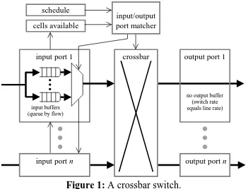
Figure 1 illustrates a crossbar switch. During each time slot the input/output port matcher evaluates the schedule and the set of flows that have cells available and decides which flows will send a cell through the crossbar in the next time slot.
Flows may be unicast flows, which must use exactly one output port of the switch, or multicast flows, which can use more than one output port. (In either case, the flow must use exactly one input port.) For the present, we consider only unicast flows. A rudimen-tary way to handle multicast flows will be discussed in Section 7.
Suppose we have a scheduling frame size of n slots and a set B of bandwidth requests, where each request has the form “flow f needs mcells per frame of bandwidth from input port ito output port o.” Given this set B of bandwidth requests, the schedule must satisfy the following two constraints to provide all the requested guarantees of service:
• Each flow must be scheduled into the requested number of slots.
• Two flows that conflict with each other by using the same input port or the same out-put port must not be scheduled into the same time slot.
frame. It turns out that this is also a sufficient condition: if no input or output port has a load of more than n cells per frame, then a legal schedule is possible [10].
input/output port matcher schedule
cells available
input buffers (queue by flow)
input port 1 crossbar output port 1
input port n output port n
[image:8.612.131.482.118.386.2]no output buffer (switch rate equals line rate)
Figure 1: A crossbar switch.
Usually, if any legal schedule exists, there are many such schedules. These schedules differ in the timing of the forwarding of cells, and, as a consequence, some of these schedules require more buffering in the switch than others require. We are interested in finding schedules that provide guarantees that allow us to build a switch with less buff-ering than would otherwise be required. In particular, we are interested in “smooth” schedules that distribute the scheduled slots so that cells of an input port, an output port, or a flow are processed at a relatively steady rate throughout the scheduling frame. Such schedules also result in lower worst-case latency than arbitrary legal schedules.
For example, suppose that the data cells of a flow arrive at the switch at a relatively steady rate, but pass through the switch according to a legal schedule in which all the scheduled slots for the flow are clustered at the end of the frame. The latency period during which cells of the flow must wait in the input buffers could be quite long—almost a frame time—and the amount of buffer space used by cells in the flow could be quite large—almost the per-frame bandwidth of the flow.
clus-tered into one part of the schedule. Then the amount of output buffering needed at each output port could approach the per-frame bandwidth of the link, and the latency intro-duced by output buffering could approach the frame time.
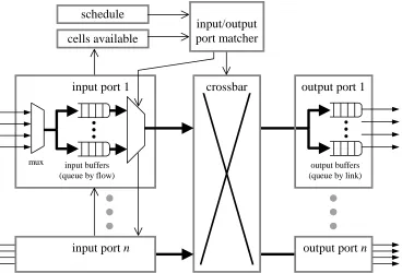
The recursively balanced scheduling method we describe below avoids the problems associated with clustering by distributing the time slots for each flow approximately uni-formly throughout the scheduling frame. The method can also ensure that the time slots during which any given output link is used are distributed approximately uniformly throughout the scheduling frame. The method can compute a schedule having both these smoothness properties regardless of the complexity of the pattern of bandwidth requests and regardless of the amount of load, provided there is no input or output port whose load exceeds the switch’s per-port bandwidth and no output link whose load exceeds the bandwidth of that link. Previously known methods for regulating switch traffic cannot simultaneously handle high loads and guarantee smoothness [3, 7, 10].
The problem of computing a schedule from a set of bandwidth requests also arises in the context of time-domain multiplexed access (TDMA) networks such as satellite com-munications systems. However, such systems take an appreciable time to reconfigure the switch, so work in this area [8, 13, 17] has concentrated on minimizing the length of the schedule and the number of distinct configurations needed rather than on smoothness. Our model assumes that reconfiguration occurs every time slot, pipelined with the data transfer, and therefore is effectively instantaneous.
input/output port matcher schedule
cells available
input buffers (queue by flow)
input port 1 crossbar output port 1
input port n output port n
mux output buffers
[image:9.612.123.491.380.630.2](queue by link)
3. The basic recursively balanced scheduling method
The input to the basic recursively balanced scheduling method consists of
• the frame size n, which must be an exact power of two, and
• a set B of bandwidth requests. Each bandwidth request b has four fields, b.f, b.i, b.o, and b.m, where
• b.f is a flow identifier, unique within B,
• b.i is the input port for b, one of in1, in2, etc.,
• b.o is the output port for b, one of out1, out2, etc., and
• b.m is the bandwidth for b, given as a non-negative integer number of cells per frame.
In Section 6 we will present modifications to the method to handle arbitrary-sized frames. Because flow identifiers are unique within B, it is unambiguous to refer to the unique bandwidth request b for flow f in B as simply B[f]. The sum of the bandwidths for all bandwidth requests in B we call the load of B. We define the load in B for a flow f, an input port i, or an output port o, as the sum of the bandwidths for all bandwidth requests with that flow, input port, or output port. In the case of a flow, there will be at most one such bandwidth request: B[f] if it exists. Table 1 summarizes the definitions.
load(B) ≡
∑
b∈Bb.m load of B load(B, f) ≡∑
= ∈Bbf f
b :. b.m load in B due to flow f load(B, i) ≡
∑
∈ =i i b B
b :. b.m load in B on input port i load(B, o) ≡
∑
b∈B:b.o=ob.m load in B on output port oTable 1: Load definitions.
The bandwidth request set B is feasible for frame size n if the load in B on each input and output port is at most n. If the bandwidth request set is not feasible, no schedule is possible. The scheduling method described below works for any feasible request set.
The output is a schedule S associating each time slot t in the range 1,,n with a set S[t] of flows. The schedule S has the following properties:
LEGAL.1. For any flow f, the number of time slots in which flow f appears in sched-ule S equals the load in B due to f. Formally,
{
t:f ∈S[t]}
=load(B,f).LEGAL.2. No two flows that use the same input or output port appear in the same time slot of S.
3.1. Recursive splitting of the scheduling frame
The recursively balanced scheduling method works by recursive splitting of the schedul-ing frame. Because the frame size is a power of two, each split divides the schedulschedul-ing frame exactly in half.
The base case of the recursion is the case n = 20 = 1; that is, there is just one slot in the frame. Since the bandwidth request set B is required to be feasible for the frame size n = 1, there can be at most one request in B for a flow of non-zero bandwidth for any given input or output port, and each such request must be for a bandwidth of 1. So the method simply returns a one-slot schedule S, where S[1] is the set of all positive-bandwidth (i.e., positive-bandwidth 1) flows in B.
The other case is that n = 2k+1 for some non-negative integer k. In this case, the method splits the bandwidth request set B into two bandwidth request sets B1 and B2 having the following properties:
SPLIT.1. Each flow f has the same input and output ports in B1 and B2 as in B. Formally,
if B1[f] exists then B1[f].i = B[f].i and B1[f].o = B[f].o, and if B2[f] exists then B2[f].i = B[f].i and B2[f].o = B[f].o.
SPLIT.2. Each flow f has its load in B divided between B1 and B2. Formally,
( )
B f load(
B1 f)
load(
B2 f)
load , = , + , .
SPLIT.3. Each flow f has its load divided as equally as possible. Formally,
(
B1,f)
−load(
B2,f)
≤1load .
SPLIT.4. Each input port i has its load divided as equally as possible. Formally,
( )
B1,i −load(
B2,i)
≤1load .
SPLIT.5. Each output port o has its load divided as equally as possible. Formally,
(
B1,o)
−load(
B2,o)
≤1load .
The method then recursively computes schedules S1 for B1 and S2 for B2, each with frame size k
n 2=2 , and concatenates those schedules to produce the schedule S for B. In order for the splitting step to be correct, B1 and B2 must each be feasible for frame size n 2=2k. Properties SPLIT.1 and SPLIT.2 imply that the port loads in B1 and B2 sum to the corresponding port loads in B. Since B is feasible for frame size n, no port load in B can exceed n. Adding properties SPLIT.4 and SPLIT.5, along with the fact that n is even, allows the conclusion that no port load in B1 or B2 will exceed n 2 . Hence B1 and B2 will indeed each be feasible for frame size n 2 .
Property SPLIT.3 leads to a per-flow smoothness property that will be discussed later. Properties SPLIT.4 and SPLIT.5, in addition to guaranteeing that the subproblems are feasible, also lead to a per-port smoothness property.
3.2. The splitting step
The splitting step can be accomplished as follows. For each bandwidth request b in B, let b1 and b2 be bandwidth requests (called subrequests of b) each with the same flow, input port, and output port as b and as nearly as possible half the bandwidth. See Table 2.
b1.f ≡ b.f b1.i ≡ b.i b1.o ≡ b.o b1.m ≡
b.m / 2
b2.f ≡ b.f b2.i ≡ b.i b2.o ≡ b.o b2.m≡
b.m / 2
Table 2: Subrequest definition.
When the bandwidth of b is odd, subrequest b1 gets half the bandwidth rounded down to an integer and b2 gets half the bandwidth rounded up. Note that b1.m+b2.m=b.m and
1 . 1 . 2
0≤b m−b m≤ .
For each bandwidth request b in B, either b1 or b2 will be allocated to B1 and the other subrequest will be allocated to B2. Any such allocation of the subrequests to B1 and B2 will make B1 and B2 satisfy properties SPLIT.1-3. It remains to describe how to allocate the subrequests so that properties SPLIT.4 and SPLIT.5 are satisfied.
For each even-bandwidth request b in B, b1 and b2 are equal, so the allocation is ar-bitrary. We will ignore even-bandwidth requests and will consider only odd-bandwidth requests for the remainder of this section.
For an odd-bandwidth request b, subrequest b2 has bandwidth greater by one cell per frame than b1. We say that b favors whichever subrequest set receives subrequest b2, the subrequest of greater bandwidth. In order to satisfy properties SPLIT.4 and SPLIT.5, we must guarantee that the following properties hold:
ALLOC.1. For each input port i, the number of odd-bandwidth requests for i favor-ing B1 and the number favorfavor-ing B2 differ by at most one.
ALLOC.2. For each output port o, the number of odd-bandwidth requests for o fa-voring B1 and the number fafa-voring B2 differ by at most one.
We will achieve these properties by reducing the problem to that of finding a 2-coloring of a certain graph.
INPAIR.1. Each request appears at most once (as a member of an input pair) in IP, and no request can be paired with itself.
INPAIR.2. If
{ }
b,c ∈IP, then b.i=c.i.INPAIR.3. For any input port i, there is at most one odd-bandwidth request for i that does not appear (as a member of an input pair) in IP.
To construct IP we simply pair off as-yet-unpaired same-input odd-bandwidth requests until there is at most one unpaired odd-bandwidth request left for each input port. Subse-quently we will allocate subrequests so that the members of each input pair favor differ-ent subrequest sets. In such an allocation, the load on any input port due to any input pair will divide exactly evenly and we say that the input pair is balanced. Since at most one request for input port i appears in no input pair, the load on i will be divided as equally as possible.
Similarly, we achieve property ALLOC.2 by forming pairs of odd-bandwidth requests that have the same output port and then allocating subrequests so that the members of a pair favor different subrequest sets. The output pairing, OP, is a set of unordered output pairs of odd-bandwidth requests. OP must satisfy the following properties:
OUTPAIR.1. Each request appears at most once in OP, and no request can be paired with itself.
OUTPAIR.2. If
{ }
b,c ∈OP, then b.o=c.o.OUTPAIR.3. For any output port o, there is at most one odd-bandwidth request for o that does not appear in OP.
We construct OP in an analogous way to IP.
To achieve both ALLOC.1 and ALLOC.2 we must allocate the subrequests so that all input pairs and output pairs are balanced simultaneously. As we will show below, this allocation problem is equivalent to finding a 2-coloring of a graph G whose vertex set is the set of odd-bandwidth requests in B and whose edge set is the (labeled) union of IP and OP. We need a labeled union because it is possible for
{ }
b,c ∈IP and{ }
b,c ∈OP, in which case there must be two edges between b and c.Observe that each vertex b in G has degree at most two: one incident edge corre-sponding to b’s membership in an input pair (if any), and one incident edge correspond-ing to b’s membership in an output pair (if any). Suppose we have a 2-colorcorrespond-ing of G us-ing the colors white and black. For each white odd-bandwidth request, allocate the subrequests to favor B1, and for each black odd-bandwidth request, allocate the subre-quests to favor B2. Now consider any input pair
{ }
b,c ∈IP. Since{ }
b,c is an edge in G, b and c must have opposite colors and hence the input pair is balanced. The same rea-soning applies to any output pair. Hence all input pairs and output pairs are balanced and we achieve both ALLOC.1 and ALLOC.2.hence vertices) around any cycle must be even. So to produce a 2-coloring, we simply traverse each path and cycle in turn, assigning alternating colors to the vertices. An ex-ample of such a coloring appears in Figure 3 in the next section.
3.3. An example of the splitting step
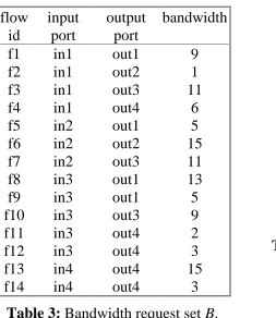
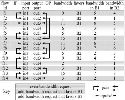
Here is an example to illustrate the splitting step. Suppose that the frame size is 32 and we have the bandwidth request set B shown in Table 3. Checking the port loads, as shown in Table 4, we see that no input or output port load exceeds 32, and thus the bandwidth request set is feasible.
We identify the bandwidth requests by their unique flow ids. The easy part of split-ting B into B1 and B2 is to deal with the even-bandwidth requests, which split exactly in half. The even-bandwidth requests are f4 and f11. Request f4 splits into two subrequests of bandwidth 3 and request f11 into two subrequests of bandwidth 1. In the final result shown in Table 5, shaded horizontal lines mark these even-bandwidth requests.
flow
id
input
port
output
port
bandwidth
f1
in1
out1
9
f2
in1
out2
1
f3
in1
out3
11
f4
in1
out4
6
f5
in2
out1
5
f6
in2
out2
15
f7
in2
out3
11
f8
in3
out1
13
f9
in3
out1
5
f10
in3
out3
9
f11
in3
out4
2
f12
in3
out4
3
f13
in4
out4
15
f14
in4
out4
3
Table 3: Bandwidth request set B.
port load
in1
27
in2
31
in3
32
in4
18
out1
32
out2
16
out3
31
[image:14.612.104.357.294.586.2]out4
29
Table 4: Port loads in B.
The hard part is to deal with the odd-bandwidth requests, namely f1–f3, f5–f10, and f12–f14. Each such request will split into two subrequests whose bandwidths differ by one cell per frame. For example, the request f1 has bandwidth 9; its subrequests will have bandwidths 4 and 5. We must decide which requests favor B1 and which favor B2.
re-quests, which we group into two pairs, {f8, f9} and {f10, f12}. Finally the two requests f13 and f14 that use in4 are paired with each other. The final input pairing is
IP = {{f1, f2}, {f5, f6}, {f8, f9}, {f10, f12}, {f13, f14}}. In the same way, we can construct an output pairing, such as
OP = {{f1, f5}, {f8, f9}, {f2, f6}, {f7, f10}, {f12, f13}}.
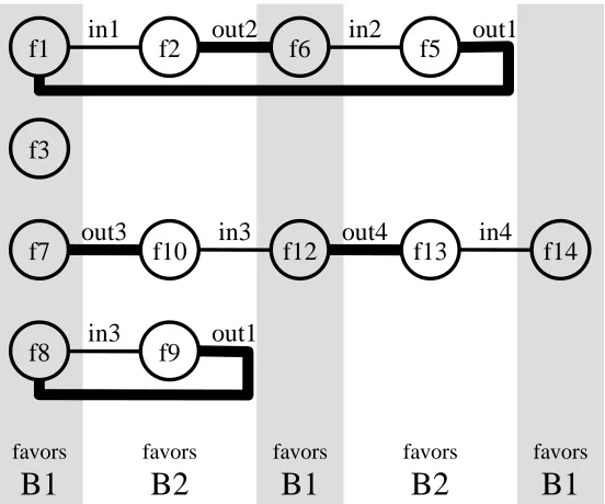
For example, f7 and f10 can be paired since they share output port out3. The only re-maining flow requesting out3 is f3, so it must remain unpaired. Figure 3 shows the paths and cycles produced by this input and output pairing. To help illustrate the fact that cy-cles must be even, edges resulting from the input pairing IP are drawn with thin lines and edges resulting from the output pairing OP are drawn with thick lines.
f1 in1 f2 out2 f6 in2 f5 out1
f3
f7
f9 f8
f10 f12 f13 f14
in3 out1
out3 in3 out4 in4
favors
B1
favors
B2
favors
B1
favors
B2
favors
[image:15.612.169.445.244.474.2]B1
Figure 3: Paths and cycles of odd-bandwidth requests.
Next we traverse the paths and cycles, alternately favoring B1 and B2. The columns in Figure 3 are shaded to show this alternation. Note that we have some freedom in whether an odd-length path on balance favors B1 or B2. If we wanted to ensure that the total load of B was divided as evenly as possible (which is not a requirement), we could do so by pairing up odd-length paths.
Combining the subrequests of the odd-bandwidth requests with the subrequests of the even-bandwidth requests already discussed, we arrive at the subrequest sets B1 and B2 shown in Table 5.
flow
id
IP
input
port
output
port
OP bandwidth favors bandwidth
in B1
bandwidth
in B2
f1
in1
out1
9
B1
5
4
f2
in1
out2
1
B2
0
1
f3
in1
out3
11
B1
6
5
f4
in1
out4
6
3
3
f5
in2
out1
5
B2
2
3
f6
in2
out2
15
B1
8
7
f7
in2
out3
11
B1
6
5
f8
in3
out1
13
B1
7
6
f9
in3
out1
5
B2
2
3
f10
in3
out3
9
B2
4
5
f11
in3
out4
2
1
1
f12
in3
out4
3
B1
2
1
f13
in4
out4
15
B2
7
8
f14
in4
out4
3
B1
2
1
even-bandwidth request
odd-bandwidth request that favors B1
odd-bandwidth request that favors B2
pairs
unpaired
[image:16.612.101.514.72.401.2]key
Table 5: Calculation of bandwidth subrequest sets B1 and B2.
port
load in
B
load in
B1
load in
B2
in1
27
14
13
in2
31
16
15
in3
32
16
16
in4
18
9
9
out1
32
16
16
out2
16
8
8
out3
31
16
15
out4
29
15
14
[image:16.612.204.409.463.628.2]Recursive splitting would divide B1 into two subframes, each having load 14/2 = 7 for in1 and load 16/2 = 8 for out1, and so on. Similarly, B2 would be divided into two subframes, where each subframe would have load 16/2 = 8 for out1 and where one sub-frame would have load (13+1)/2 = 7 for in1 and the other subsub-frame would have load (13-1)/2 = 6 for in1. Five levels of recursive splitting will split B into 32 request sets such that no port has load greater than 1 in any single request set. At that point the switch can satisfy the requests during a single time slot.
This completes the description of the basic recursively balanced scheduling method.
4. Degree of smoothness achieved by the basic method
Smooth schedules were described above as ones in which the scheduled time slots for each flow are approximately uniformly distributed throughout the duration of the sched-uling frame. Here is a quantitative characterization of the sense in which recursively bal-anced schedules are smooth.
Suppose we have a schedule S for a frame of size n. For some flow or port whose load is of interest, the question is: How is the load spread out over the schedule? Let the load be m cells per frame. Some slots in S contain a unit of the load and the other slots contain no load. From the point of view of the flow or port, the slots in S that contain a unit of load are full and the rest are empty.
Now let S* be the schedule produced by concatenating an unlimited number of repe-titions of S and consider any interval I consisting of I consecutive slots from S*. De-fine the perfect load in I, P
( )
I , as I m n and the scheduled load in I, S( )
I , as the num-ber of full slots in I. If the schedule were perfectly smooth, then we would expect( ) ( )
I S IP = . This cannot usually be achieved, if only because slots are discrete and I m n may not be an integer. We define the scheduling discrepancy (with regard to a flow or port) over interval I as S
( ) ( )
I −P I . We define the maximum scheduling dis-crepancy in S, msd( )
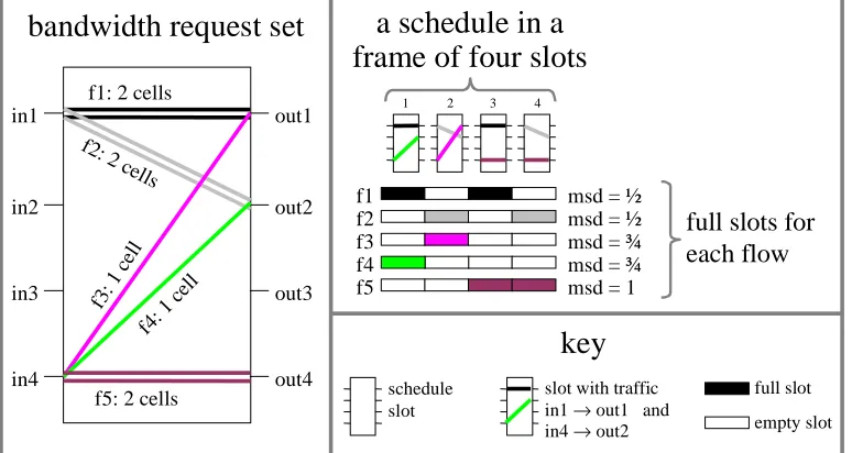
S , as the maximum scheduling discrepancy over any interval I from S*.leaves f5 with one even-numbered and one odd-numbered slot, resulting in a maximum scheduling discrepancy of 1 for f5.
flow
id
input
port
output
port
bandwidth
f1
in1
out1
2
f2
in1
out2
2
f3
in4
out1
1
f4
in4
out2
1
[image:18.612.199.415.124.239.2]f5
in4
out4
2
Table 7: A bandwidth request set with no all-min-msd
schedule in a frame of four slots.
key
schedule slot
slot with traffic in1 → out1 and in4 → out2
bandwidth request set
a schedule in a
frame of four slots
f1 f2 f3 f4 f5
msd = ½ msd = ½ msd = ¾ msd = ¾ msd = 1
full slots for each flow
full slot empty slot
f1: 2 cells
f2: 2 c ells
f3: 1 cel
l
f4: 1 cel
l
f5: 2 cells in1
in2
in3
in4
out1
out2
out3
out4
1 2 3 4
Figure 4: A four-slot schedule for the bandwidth request set of Table 7.
Since an operational system recomputes the schedule from time to time as flows are added or removed, we extend the definition of scheduling discrepancy to a concatenation in which the schedules need not all be identical. Given a set SS of schedules, we define the maximum scheduling discrepancy in SS, msd
( )
SS , as the maximum scheduling dis-crepancy over any interval I from any concatenation of schedules from SS. We are par-ticularly interested in sets of recursively balanced schedules, although for comparison we also consider sets of all legal schedules. [image:18.612.115.502.298.504.2]load of m cells per frame has been split in half over and over again as equally as possible. Using this property we will obtain bounds on msd
( )
RBn and msd(
RBn,m)
.In Section 4.1 we give a method and example of calculating the maximum scheduling discrepancy in any given schedule S. In Section 4.2 we compute the value of msd
( )
LSn by considering pathological but legal schedules. Generalizing the method of Section 4.1 and applying the smoothness property of recursively balanced schedules, in Section 4.3 we obtain a bound on msd( )
RBn when n is a power of two. In Section 4.4 we compare this bound with some actual values of msd(
RBn,m)
.4.1. Maximum scheduling discrepancy in a given schedule
Suppose we have a scheduling frame of size n and a flow or port with a load m. The maximum scheduling discrepancy in any given schedule S for this situation can be callated as follows. First we construct two functions from cumulative (elapsed) slots to cu-mulative cells. The cucu-mulative scheduled load function S(t) is a bumpy line with a slope of 0 during each empty slot and a slope of 1 during each full slot. The cumulative perfect load function P(t) is a straight line with a slope of m n . Both S and P start at
) 0 , 0
( and end at ( mn, ): S(0)=P(0)=0 and S(n)=P(n)=m. Next we compute the difference D(t)≡S(t)−P(t). The difference between the extreme high and low values of D is the maximum scheduling discrepancy in the schedule S. The interval that exactly spans the times at which the extreme high and low values of D occur has this discrep-ancy, and no interval has a greater discrepancy. Note that this calculation applies to any schedule, regardless of whether or not it is recursively balanced.
An example will illustrate the calculation. Figure 5 shows a construction of a recur-sively balanced schedule for frame size n=16 and load m=10 . Note that each time the load splits, the division is as equal as possible; hence the schedule is recursively balanced. Full slots are shaded in and empty slots are shown empty.
Figure 6 shows the cumulative scheduled load function S and cumulative perfect load function P for this schedule.
The difference D ≡ −S P is plotted in Figure 7. An interval I of consecutive slots can be represented by its beginning and ending cumulative slot values, say t0 and t1. Note
that t1− =t0 I . Observe that S(t1)−S(t0) is exactly the number of full slots in I and P t( )1 −P t( )0 = I m n. Hence the scheduling discrepancy over I is D t( )1 −D t( )0
.
1 1 1 2 2 1 1 1
2 3 3 2
5 5
10
0 1 1 0 0 1 1 1 1 1 1 0 1 0 1 0
0
1
2
3
4
24
23
22
21
20 slots in subframe recursion
[image:20.612.154.515.65.564.2]level
Figure 5: A recursively balanced schedule
for load 10 in frame size 16.
cumulative slots
0
c
u
mul
ative cells
schedule
perfect load scheduled load
S
P
Figure 6: Scheduled load and perfect load for one
frame of a recursively balanced schedule.
D
0
cumulative slots
∆
c
ells
d
I
[image:20.612.190.517.75.329.2]calculation of discrepancy d over interval I
[image:20.612.171.486.590.679.2]4.2. Maximum scheduling discrepancy in legal schedules
In this section we compute msd
( )
LSn , the maximum scheduling discrepancy in any con-catenation of legal schedules of any loads in frames of size n. First, let us consider legal schedules of load m. Since D ≡ −S P, the highest possible value of D results from packing the entire load into the initial slots of the scheduling frame and evaluating at time m. Using the subscript m to indicate this schedule, we have( )
m mSm = ,
( )
m m m n Pm = ⋅ , and( ) (
m m n m m)
nDm = ⋅ − ⋅ .
Next, keeping the frame size fixed at n, Dm
( )
m is maximized when m=n 2. Hence, for any time t in any legal schedule for any load in a frame of size n,( )
t n 4D ≤ ,
and this bound is tight. A symmetrical argument packing the entire load into the final slots of the scheduling frame bounds D from below. Hence, the maximum scheduling discrepancy in any concatenation of legal schedules with a frame of size n is n 2. For-mally,
( )
LS n 2msd n = .
For example, suppose we have a 1024-slot scheduling frame (n = 1024). Then the maximum scheduling discrepancy in any concatenation of legal schedules is 512 cells. This maximum is attained in the case of a load of 512 cells per frame and two consecu-tive scheduling frames. In the first frame all 512 cells of the load appear in the final 512 slots of the frame, leaving the initial 512 slots empty. In the second frame (presumably due to an unfortunate scheduling change) all 512 cells of the load appear in the initial slots of the frame, leaving the final 512 slots empty. The 1024-slot interval consisting of the final 512 slots of the first frame and the initial 512 slots of the second frame has a scheduled load of 1024 and a perfect load of 512, for a discrepancy of 512 cells.
Although the recursively balanced scheduling method does not necessarily minimize the maximum scheduling discrepancies of all flows and ports, the discrepancies it pro-duces are much smaller than the maximum scheduling discrepancies of schedules that are legal but satisfy no additional smoothness requirements. Consider again a 1024-slot scheduling frame. In the following section, we will show that the maximum scheduling discrepancy in any concatenation of 1024-slot recursively balanced schedules of any loads cannot exceed 6.89 cells. This is much better than the 512 cell maximum discrepancy in legal schedules.
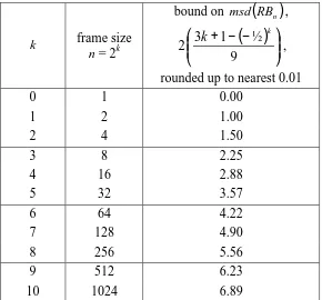
4.3. A bound for msd in recursively balanced schedules
( )
( )
( )
− − + = + − − ≤ 9 ½ 1 2 3 2 9 ½ 1 3 2 2 k k k k RBmsd k .
That is, in any concatenation of recursively balanced 2 -slot scheduling frames of anyk loads, the scheduling discrepancy over any interval is at most 2k 3+εk cells, where
3 1 0≤εk ≤ .
Consider a concatenation of recursively balanced 2 -slot scheduling frames. Letk k
n=2 be the number of slots in a frame. Recall the definitions of S
( )
t , P( )
t , and D( )
t from Section 4.1. Note that P( )
t has constant slope during a frame. Our analysis de-pends on finding bounds for D( )
t .Since each whole scheduling frame has the correct number of slots allocated for its load, it follows that at each frame boundary—that is, whenever t is an integer multiple of the frame size n—we have S
( ) ( )
t =P t , and thus D( )
t =0.The recursively balanced scheduling method proceeds by splitting the frame into smaller and smaller subframes. Let us consider any frame or subframe F starting at time
0
t and ending at time at t , where 1 t1−t0 ≥2. F contains t1−t0 slots. The defining smoothness property of a recursively balanced schedule is that the load in each half of F differs from half of the load of F by at most half a cell. In particular, the load in the first half of F can be no greater than half the load of F plus half a cell:
( )
( ) ( )
2 1 2 0 1 0 01 − ≤ − +
− S t S t
t S t t S , or equivalently
( ) ( )
2 1 2 0 1 01 ≤ + +
−t t S t S t
S .
Within a frame, P
( )
t has constant slope. So we have( ) ( )
2 2 0 1 01 t P t P t t
P = +
− .
Hence we can bound the value of D at the midpoint of F:
− − − = − 2 2 2 0 1 0 1 0
1 t t
P t t S t t D
( ) ( )
( ) ( )
2 2 1S t1 +S t0 + − P t1 +P t0
≤
( ) ( ) ( ) ( )
2
1 1 − 1 + 0 − 0 +
= S t P t S t P t
( ) ( )
2
1 1 + 0 +
Let i and j be integers, where 0≤i≤k. Observe that any time of the form j2k−i is the boundary of a subframe of size 2k−i. Let us define Di as the maximum value of D at any boundary of a subframe of size 2k−i. Formally,
( )
{
k i}
j
i D j
D ≡max 2 − .
Now any time of the form j2 is a frame boundary, hencek 0
0 =
D .
Any time of the form j2k−1 is either a frame boundary (for which D has value 0) or the midpoint of a frame (for which, from the midpoint inequality above, D has value at most
(
0+0+1)
2). Hence2 1 1 ≤
D .
For 2≤i≤k, any time of the form j2k−i can be characterized based on whether j is even or odd. If j is even, j2k−i is an integer multiple of 2k−( )i−1 . If j is odd, j2k−i is the mid-point of a subframe whose starting and ending times are successive integer multiples of
( )1
2k−i− , one of which is necessarily an integer multiple of 2k−( )i−2 . Hence, for 2≤i≤k,
+ + ≤ − − − 2 1 , max 1 2 1 i i i i D D D D .
From the above recurrence, it follows (as can readily be checked) that
( )
9 ½ 1 3 i i iD ≤ + − − ,
for any integer i in the range 0≤i≤k. Taking i=k, we have
( )
( )
9 ½ 1 3 k k k D tD ≤ ≤ + − − ,
for any integer t, and thus for any time t whatsoever. (Since both S and P have constant slope within any single slot, the maximum value of D must occur at a slot boundary.)
By a symmetrical argument, D is bounded below by
( )
( )
9 ½ 1 3 k k tD ≥ − + − − ,
and the bound on maximum scheduling discrepancy claimed at the start of this section,
( )
≤ + −( )
− 9 ½ 1 3 2 2 k k RBmsd k ,
follows immediately.
bal-anced schedule of this frame size. As expected, 2.25 does not exceed the theoretical bound of 2.88.
As discussed later in Section 7, our switch implementation uses a frame size of 1024 slots. From Table 8 we see that the maximum scheduling discrepancy in recursively bal-anced schedules of this frame size cannot exceed 6.89 cells.
k frame size n = 2k
bound on msd
( )
RBn ,( )
+ − −
9 ½ 1 3 2
k k
,
rounded up to nearest 0.01
0 1 0.00
1 2 1.00
2 4 1.50
3 8 2.25
4 16 2.88
5 32 3.57
6 64 4.22
7 128 4.90
8 256 5.56
9 512 6.23
[image:24.612.162.452.164.434.2]10 1024 6.89
Table 8: Bound on msd(RB
n) for various frame sizes.4.4. Actual msd values for certain loads
Recall that we have a scheduling frame of size n=2k and a flow or port of interest whose load is m. In the previous section we obtained a bound for msd
( )
RB2k , the maximumscheduling discrepancy in any concatenation of recursively balanced k
2 -slot scheduling frames of any loads. For a given load m, the maximum scheduling discrepancy
(
RBkm)
msd ,
2 could be much less than the bound.
In general, the worst case discrepancy for any given load occurs when a frame with its load scheduled as late as permissible (called a latest-load frame) is followed—after zero or more intervening frames—by a frame with its load scheduled as early as permissible (an earliest-load frame). A latest-load frame achieves the minimum possible value of
( )
tD and an earliest-load frame the maximum possible value. Some other schedules may also achieve these extremal values, but none can exceed them.
( )
− = k k RB msd 2 1 1 2 1 , 2 .The latest-load frame has its last slot full, and the earliest load frame has its first slot full.
When m is a power of 2, say m=2a, we have
(
)
2 2 1 1 2 2 ,2 <
− = k−a
a k
RB
msd .
Any recursively balanced schedule for this load puts one cell of load into each 2k−a-slot subframe. This is exactly the same situation as a load of 1 in a frame of size 2k−a.
Now suppose m is a sum of two distinct powers of 2, say m=2a +2b, with a<b. Observe that the full slots in any recursively balanced schedule can be partitioned into two sets A and B, where A is the set of full slots in some recursively balanced schedule of load 2 and B is the set of full slots in some recursively balanced schedule of load a 2 .b Hence,
(
RBk a b)
msd(
RB k a)
msd(
RBk b)
msd 2 , 2 2 , 2 2 2 ,
2 + ≤ + .
4 2 2 1 2 2 1 2 < − + −
= ka kb .
This bound is not tight because, for example, A and B cannot both contain the first slot of any subframe. In fact, the worst case discrepancy is
(
)
− − + − = + b a k b k a b a k RB msd 2 2 2 2 1 2 2 1 2 2 2 , 2 .The latest-load frame has two full slots in its last 2k−b-slot subframe and a full slot as the last slot of its next-to-last 2k−b-slot subframe, making a total of three cells of load in the last 2k−b+1 slots of the frame. A symmetrical situation occurs at the beginning of the earliest-load frame.
Although it is beyond the scope of this report to give a complete analysis, maximum scheduling discrepancies are small for loads which are sums and differences of a small number of powers of two.
As discussed later in Section 7, our switch implementation uses a frame size of 1024 slots. Table 9 gives maximum scheduling discrepancies for arbitrary concatenations of recursively balanced schedules of any given load m=a+b with frame size 1024. We show the msd values only for loads up to a few more than 512. Values for higher loads can be found by symmetry: because the full slots in an earliest-load frame of load m are precisely the empty slots in a latest-load frame of load n−m, and vice versa,
(
RBnm)
msd(
RBnn m)
msd , = , − .
b 0 1 2 3 4 5 6 7 8 9 10 11 12 13 14 15
a 00002 00012 00102 00112 01002 01012 01102 01112 00002 10012 10102 10112 11002 11012 11102 11112
0 02 0.00 2.00 2.00 2.99 1.99 3.49 2.99 3.49 1.98 3.73 3.48 4.23 2.98 4.22 3.47 3.72
16 100002 1.97 3.84 3.71 4.59 3.46 4.83 4.21 4.58 2.95 4.58 4.20 4.82 3.45 4.57 3.69 3.81
32 1000002 1.94 3.87 3.81 4.74 3.68 5.12 4.55 4.99 3.42 5.11 4.79 5.48 4.16 5.35 4.54 4.72
48 1100002 2.91 4.72 4.53 5.34 4.15 5.46 4.77 5.08 3.39 4.95 4.51 5.07 3.63 4.69 3.75 3.81
64 10000002 1.88 3.84 3.81 4.78 3.74 5.21 4.68 5.14 3.61 5.33 5.04 5.76 4.48 5.69 4.91 5.13
80 10100002 3.34 5.19 5.03 5.87 4.71 6.05 5.39 5.74 4.08 5.67 5.26 5.85 4.45 5.54 4.63 4.72
96 11000002 2.81 4.72 4.62 5.53 4.43 5.83 5.24 5.64 4.05 5.70 5.36 6.01 4.66 5.82 4.97 5.13
112 11100002 3.28 5.06 4.84 5.62 4.40 5.68 4.96 5.24 3.52 5.04 4.57 5.10 3.63 4.66 3.69 3.72
128 100000002 1.75 3.73 3.71 4.70 3.68 5.16 4.64 5.13 3.61 5.34 5.07 5.81 4.54 5.77 5.00 5.24
144 100100002 3.47 5.33 5.18 6.04 4.90 6.26 5.61 5.97 4.33 5.94 5.54 6.15 4.76 5.87 4.97 5.08
160 101000002 3.19 5.11 5.03 5.95 4.87 6.29 5.71 6.13 4.55 6.22 5.89 6.56 5.23 6.40 5.57 5.74
176 101100002 3.91 5.70 5.50 6.29 5.09 6.38 5.68 5.97 4.27 5.81 5.36 5.90 4.45 5.49 4.54 4.58
192 110000002 2.63 4.58 4.53 5.48 4.43 5.88 5.33 5.78 4.23 5.94 5.64 6.34 5.04 6.24 5.44 5.64
208 110100002 3.84 5.67 5.50 6.32 5.15 6.47 5.80 6.13 4.45 6.03 5.61 6.18 4.76 5.83 4.91 4.99
224 111000002 3.06 4.95 4.84 5.73 4.62 6.01 5.39 5.78 4.17 5.81 5.45 6.09 4.73 5.87 5.00 5.14
240 111100002 3.28 5.04 4.81 5.57 4.34 5.60 4.86 5.13 3.39 4.90 4.42 4.93 3.45 4.46 3.47 3.49
256 1000000002 1.50 3.49 3.48 4.47 3.46 4.95 4.44 4.93 3.42 5.16 4.90 5.64 4.38 5.62 4.86 5.10
272 1000100002 3.34 5.21 5.07 5.94 4.80 6.17 5.54 5.90 4.27 5.88 5.50 6.11 4.73 5.84 4.96 5.07
288 1001000002 3.19 5.12 5.04 5.97 4.90 6.33 5.75 6.18 4.61 6.29 5.96 6.64 5.32 6.50 5.68 5.85
304 1001100002 4.03 5.83 5.64 6.44 5.24 6.54 5.85 6.15 4.45 6.01 5.56 6.11 4.66 5.72 4.77 4.82
320 1010000002 2.88 4.83 4.79 5.75 4.71 6.17 5.63 6.09 4.55 6.26 5.96 6.67 5.38 6.59 5.80 6.01
336 1010100002 4.22 6.05 5.89 6.72 5.55 6.89 6.22 6.56 4.89 6.47 6.06 6.64 5.23 6.31 5.39 5.48
352 1011000002 3.56 5.46 5.36 6.25 5.15 6.54 5.94 6.34 4.73 6.38 6.03 6.67 5.32 6.47 5.61 5.76
368 1011100002 3.91 5.68 5.45 6.22 4.99 6.26 5.54 5.81 4.08 5.60 5.12 5.64 4.16 5.19 4.21 4.23
384 1100000002 2.25 4.22 4.20 5.17 4.15 5.62 5.10 5.57 4.05 5.77 5.50 6.22 4.95 6.17 5.39 5.62
400 1100100002 3.84 5.69 5.54 6.39 5.24 6.59 5.94 6.29 4.64 6.24 5.84 6.44 5.04 6.14 5.24 5.34
416 1101000002 3.44 5.35 5.26 6.17 5.09 6.50 5.91 6.32 4.73 6.40 6.06 6.72 5.38 6.54 5.71 5.87
432 1101100002 4.03 5.82 5.61 6.39 5.18 6.47 5.75 6.04 4.33 5.87 5.40 5.94 4.48 5.51 4.55 4.59
448 1110000002 2.63 4.57 4.51 5.46 4.40 5.84 5.29 5.73 4.17 5.87 5.56 6.25 4.95 6.14 5.33 5.53
464 1110100002 3.72 5.54 5.36 6.17 4.99 6.31 5.63 5.95 4.27 5.83 5.40 5.97 4.54 5.61 4.68 4.74
480 1111000002 2.81 4.69 4.57 5.46 4.34 5.72 5.10 5.48 3.86 5.49 5.12 5.75 4.38 5.51 4.64 4.78
496 1111100002 2.91 4.66 4.42 5.17 3.93 5.19 4.44 4.70 2.95 4.46 3.96 4.47 2.98 3.98 2.99 2.99
512 10000000002 1.00 2.99 2.99 3.98 2.98 4.47 3.96 4.46 2.95 4.70 4.44 5.19 3.93 5.17 4.42 4.66
Table 9: Values of msd(RB
1024,a+b), rounded to the nearest 0.01.Because msd
(
RB2n,2m)
=msd(
RBn,m)
, Table 9 can also be used to look up the maxi-mum discrepancy values for any given load in a k2 -slot frame, where 2k <1024. For example, for a load of 21 cells and a frame size of 64 slots, we have
(
RB21,64)
=msd(
RB16×21,16×64)
=msd(
RB336,1024)
≈4.22msd .
Note that this value, being the largest in the first column of the table, is the worst-case maximum scheduling discrepancy for any load in a 64-slot frame.
5. Output link smoothness
The basic recursively balanced scheduling method can be extended to achieve per-output-link smoothing. We modify each bandwidth request b by replacing the output port field b.o with an output link field b.ol that gives the specific output link. All references to output port b.o are interpreted by mapping output link b.ol to the output port that contains it. We define load(B, ol), the load in B on output link ol, as the sum of the bandwidths for all bandwidth requests with output link ol:
load(B, ol) ≡
∑
∈ = ol ol b Bb :. b. .m
Note that a feasible schedule is not possible if any output link is overloaded. To the properties SPLIT.1-5 from Section 3.1 we add the following properties:
SPLIT.6. Each flow f has the same output link in B1 and B2 as in B. Formally, if B1[f] exists then B1[f].ol = B[f].ol, and
if B2[f] exists then B2[f].ol = B[f].ol.
SPLIT.7. Each output link ol has its load divided as equally as possible. Formally,
(
B1,ol)
−load(
B2,ol)
≤1load .
Property SPLIT.6 amplifies SPLIT.1 to guarantee that the splitting step preserves each flow’s output link. Property SPLIT.7 guarantees per-output-link smoothness. Note that SPLIT.7 does not supersede property SPLIT.5. Dividing the load on each output link as equally as possible does not by itself guarantee that the load on each output port will be divided as equally as possible, which is what SPLIT.5 requires. The problem is that each of the output links of the same output port could favor the same subrequest set, leading to an excessive imbalance in the division of the load on the output port.
The enhanced properties SPLIT.1-7 can be satisfied by refining the way in which the output pairing OP is computed. Define the output link pairing, OLP, as the subset of OP in which the members of a pair have the same output link:
{ }
{
b c OP bol col}
OLP≡ , ∈ : . = . .
In addition to properties OUTPAIR.1-3 we require:
OUTPAIR.4. For any output link ol, there is at most one odd-bandwidth request for ol that does not appear in OLP.
Such a pairing may be found by first pairing requests that share output links until each output link has at most one unpaired request, then pairing as-yet-unpaired requests that share output ports until each output port has at most one unpaired request.
many cells as the number of full cells in I may arrive at the output buffer. Hence )
(RBn,m
msd bounds the difference that must be absorbed in the output buffer.
6. Odd-size frames
The recursively balanced scheduling method described above uses a splitting step that splits the bandwidth request set for an even-size frame into subrequest sets for two equal sized subframes. Since the splitting step is applied recursively, the size of each subframe to be split must also be even. Hence, as given, the method applies only to frames whose size (in slots) is an integral power of two. At the cost of losing some smoothness in the resulting schedules, the method can be extended to schedule frames of arbitrary size by generalizing the splitting step to apply to odd-size frames.
Being able to handle arbitrary-size frames is useful for several reasons. It might be desirable to use a non-power-of-two frame in order to support certain exact bandwidth requirements. Even in the case of a power-of-two frame, it might be desirable to reserve some slots throughout the schedule for other purposes, thus in effect leaving a non-power-of-two frame for the recursively balanced scheduling method. For example, slots might be reserved in order to handle multicast traffic, as in our implementation described in Section 7.
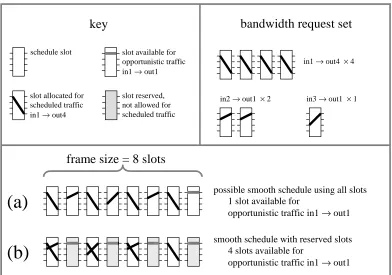
Another reason for reserving slots would be to improve the performance of opportun-istic traffic by leaving some slots completely free of scheduled traffic. This is a fairly in-teresting effect. The smooth schedule (by design) spreads its port usage throughout the slots it uses. This tends to increase the probability that a cell of opportunistic traffic will find either its input port or its output port in use in any given slot. By reserving some slots, the scheduled traffic is compressed into fewer slots, thus making it more likely that opportunistic cells can be forwarded.
Figure 8 shows an example of this effect in a frame of 8 slots. The bandwidth request set uses in1 four times and out1 three times. Case (a) shows a smooth schedule in which these uses are spread out over seven slots, leaving only one slot available for opportunis-tic traffic from in1 to out1. Although this schedule is pathological from this point of view, it is certainly a perfectly fine smooth schedule and it could have been produced by the recursively balanced scheduling algorithm. In case (b), four slots have been reserved for opportunistic traffic. The bandwidth request set is feasible for the remaining frame of four slots, so a smooth schedule can be constructed. In this case the four reserved slots are available for opportunistic traffic from in1 to out1.
To split a bandwidth request set B into a frame F of odd size 2k+1, we proceed as follows:
1. Split the frame F into three subframes, F1, F2, F3, where F1 and F3 have size k and F2 consists of a single slot.
2. Allocate one slot’s worth of sufficiently many non-conflicting flows to the single-slot subframe F2 so that the remaining requests are feasible for 2k single-slots.
key
slot available for opportunistic traffic in1 → out1
slot reserved, not allowed for scheduled traffic schedule slot
slot allocated for scheduled traffic in1 → out4
possible smooth schedule using all slots 1 slot available for
opportunistic traffic in1 → out1
bandwidth request set
in1 → out4 × 4
in2 → out1 × 2 in3 → out1 × 1
smooth schedule with reserved slots 4 slots available for
opportunistic traffic in1 → out1
(a)
(b)
[image:29.612.110.502.69.344.2]frame size = 8 slots
Figure 8: Reserving slots can improve the
performance of opportunistic traffic.
The flows assigned to F2 in step 2 may be simply the flows assigned to any single slot of any legal (not necessarily smooth) schedule for the bandwidth request set B in 2k+1 slots. One way of obtaining such a set of flows is to compute a maximum matching [4, pp. 600-604] in the bipartite graph whose vertices are the input ports and output ports of the switch and whose edges are those input-output pairs for which there is at least one positive bandwidth flow. Our implementation uses a different method, described in Sec-tion 7.5.
7. Implementation
We have implemented the recursively balanced scheduling method as part of the control software on the AN2 switch [1, 14, 16]. An AN2 network has been in daily use as a service network at our laboratory, the Digital Equipment Corporation Systems Research Center, since the end of 1994.
7.1. Hardware description
The AN2 switch hardware provides two service classes: scheduled and opportunistic. Scheduled traffic has absolute priority and is sent across the crossbar according to a schedule provided by software. The AN2 schedule frame contains 1024 cell slots. Each slot contains an entry for each of the sixteen input ports listing which virtual circuit has priority in that schedule slot from that input port. The scheduling software must guaran-tee that there is no collision of output ports. If the listed virtual circuit has no cells avail-able, its input and output ports remain available for opportunistic traffic. Schedule slots for an input port are left unused by listing virtual circuit zero, which never has cells. Op-portunistic traffic is sent across the crossbar on a best-effort basis with hardware match-ing of available input and output ports [15]. To avoid head-of-line blockmatch-ing [11], each input port maintains separate cell queues for each output port.
Each AN2 switch port accommodates an input/output line card that interfaces the switch port to one or more external communication links. The quad line card supports four SONET OC-3c links, multiplexing input cells to the switch port and demultiplexing output cells. A SONET OC-3c link (so-called 155 Megabits/second) carries 353 Kilo-cells/second. A line card that supports a single SONET OC-12 link has been developed [5], but none of these are installed at our laboratory.
Each link on the quad line card contains a small FIFO output buffer for the purpose of matching the high cell-rate output of the switch port to the slower link rate. Ten cells of storage in each FIFO are dedicated to scheduled traffic. Whenever a speed-matching FIFO gets too full, the switch hardware automatically blocks opportunistic traffic destined to that output link (causing it to queue up in the switch’s input buffers). In order to pro-vide guaranteed service, the hardware never blocks scheduled traffic. Hence the schedule must be approximately smooth with respect to each output link or else the scheduled traf-fic could overrun its dedicated storage.
A scheduled virtual circuit can forward cells simultaneously to multiple output ports and links. This is how the switch hardware supports multicast. The hardware does not support multicast for opportunistic traffic.
7.2. Software environment
The switch control software maintains a list of all scheduled virtual circuits, listing for each such circuit the input port, the output link, and the required bandwidth in cells per frame. (The output port number can be determined algebraically from the output link number.) A special output link value is used to indicate a multicast circuit. A multicast circuit that sends to all output links is full broadcast; if it sends to a proper subset there may be output ports that it does not use. Although one could exploit a multicast circuit’s unused output ports, our current system software does not do so. We treat all multicast circuits as if they were full broadcast when constructing the schedule. This also allows multicast circuits to add and drop output links without requiring the schedule to be modi-fied. We do not expect that multicast traffic will find heavy use in the network. Some heuristics are known for scheduling multicast circuits under the TDMA model [3].
scheduled circuits would not exceed a software implementation limit. The admission test guarantees that the processing step will succeed. The software limit arises from the structure of our current implementation, which uses a preallocated working store and pro-cesses each scheduled virtual circuit as a separate flow in the recursively balanced sched-uling algorithm. Preallocating the working store guarantees enough space to handle a certain number of flows. In Section 8.2 we discuss how we might aggregate flows to eliminate this software limit.
Once a batch of requests is admitted, it is processed by constructing a new list of scheduled virtual circuits (the bandwidth request set), running the recursively balanced scheduling algorithm on it, and installing the resulting, “new” schedule in the switch hardware. For difficult cases with many scheduled circuits, the scheduling algorithm can take a long time: up to a little more than a second in our current implementation. The switch hardware continues to forward cells according to the “old” schedule until the new schedule is complete, at which point the hardware flips from old to new at the next frame boundary. Processing requests in batches allows the software to support a high rate of circuit add/delete requests, although possibly at a latency of a couple of seconds. There is no difficulty in handling large batches because the recursively balanced scheduling algo-rithm always recomputes the entire schedule from scratch.
7.3. Implementation overview
The recursively balanced scheduling algorithm works by recursively splitting the problem in half, dividing the frame into two subframes and the bandwidth request set into two cor-responding sets of subrequests at each level. We implement the algorithm directly using a recursive subroutine. The implementation uses three main data structures: a schedule array indexed by input port and frame slot, a bandwidth request array, and a request-matching table.
The schedule array constitutes the result of the scheduling algorithm. As shown in Figure 9, it is a two-dimensional array whose rows correspond to input ports, whose col-umns correspond to slots in the scheduling frame, and whose entries are small integers (virtual circuit indexes) identifying flows. Initially all elements in this array are set to zero, which represents an empty schedule slot. When the recursive subroutine reaches a subframe containing one slot, it fills in the slot in the schedule array based on the surviv-ing subrequests. Because the initial problem is feasible and each step divides the problem into two feasible subproblems, we know that the final one-slot problem is feasible, which means that the surviving subrequests have a bandwidth of one cell each and no conflicts in the input or output ports. Subframes in the schedule are identified by starting slot in-dex and count.
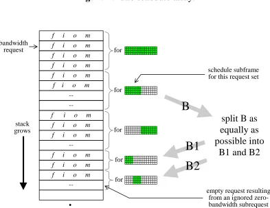
The bandwidth request array is organized as stack of request sets. At each recursive splitting step, two request sets are added to the stack. See Figure 10. This array is ini-tialized with the set of input requests and provides working storage for the splitting of one set into two sets of subrequests. A set of requests is identified by its starting index and count.
two tables, one indexed by input port and one by output link. Initially these tables are empty, represented by setting all elements to the impossible index value –1. During the splitting step the requests are scanned and each request with an odd bandwidth has its in-dex recorded in the matching tables according to its input port and output link. A match is discovered if an entry was present already in the matching table, in which case the entry is removed and the request and its match are linked together. Linking is accomplished using two extra fields per request, one for the input partner and one for the output partner. At the beginning of the splitting step, the partner fields are initialized to the impossible index value –1, again representing empty. When matches are discovered, the matching requests are linked to each other using the input or output partner field, whichever ap-plies.
input port
slot
12 12
17 6
3 7
75 2
8
3 3
75 8 17
[image:32.612.181.439.261.334.2]2
Figure 9: The schedule array.
f i o m
f i o m f i o m
f i o m
f i o m f i o m
--f i o m
--f i o m
--f i o m
--f i o m
bandwidth request
for
for
split B as
equally as
possible into
B1 and B2
B
B1
B2
stack grows
f i o m
for
f i o m
for for
empty request resulting from an ignored zero-bandwidth subrequest schedule subframe for this request set
[image:32.612.108.501.355.658.2]