WRL 95 5 pdf

WRL

Research Report 95/5

Network Behavior

of a Busy Web Server

and its Clients

research relevant to the design and application of high performance scientific computers. We test our ideas by designing, building, and using real systems. The systems we build are research prototypes; they are not intended to become products.

There are two other research laboratories located in Palo Alto, the Network Systems Lab (NSL) and the Systems Research Center (SRC). Another Digital research group is located in Cambridge, Massachusetts (CRL).

Our research is directed towards mainstream high-performance computer systems. Our prototypes are intended to foreshadow the future computing environments used by many Digital customers. The long-term goal of WRL is to aid and accelerate the development of high-performance uni- and multi-processors. The research projects within WRL will address various aspects of high-performance computing.

We believe that significant advances in computer systems do not come from any single technological advance. Technologies, both hardware and software, do not all advance at the same pace. System design is the art of composing systems which use each level of technology in an appropriate balance. A major advance in overall system performance will require reexamination of all aspects of the system.

We do work in the design, fabrication and packaging of hardware; language processing and scaling issues in system software design; and the exploration of new applications areas that are opening up with the advent of higher performance systems. Researchers at WRL cooperate closely and move freely among the various levels of system design. This allows us to explore a wide range of tradeoffs to meet system goals.

We publish the results of our work in a variety of journals, conferences, research reports, and technical notes. This document is a research report. Research reports are normally accounts of completed research and may include material from earlier technical notes. We use technical notes for rapid distribution of technical material; usually this represents research in progress.

Research reports and technical notes may be ordered from us. You may mail your order to:

Technical Report Distribution

DEC Western Research Laboratory, WRL-2 250 University Avenue

Palo Alto, California 94301 USA

Reports and technical notes may also be ordered by electronic mail. Use one of the fol-lowing addresses:

Digital E-net: JOVE::WRL-TECHREPORTS

Internet: [email protected]

UUCP: decpa!wrl-techreports

To obtain more details on ordering by electronic mail, send a message to one of these addresses with the word ‘‘help’’ in the Subject line; you will receive detailed instruc-tions.

a Busy Web Server and its Clients

Jeffrey C. Mogul

October, 1995

Abstract

The 1994 California Election server, which provided ‘‘live’’ election returns, handled over 1.5 million individual requests, including almost 1 mil-lion in a single 24-hour period. This may have been the most intensive single event on the Internet, to date, and so represented a novel experiment in how the network responds to heavy loads. We collected comprehensive traces and logs of server and network operation, allowing offline analysis of numerous statistics. This paper reports the results.

2. Overview of the Election Server 1

2.1. Content 2

2.2. Privacy 3

3. Hardware and software configuration 3

3.1. Network configuration 3

3.2. Server hardware 4

3.3. Server software 4

3.4. Log and trace collection 5

4. Overall server statistics 7

4.1. Server resource usage 9

4.2. Relative popularity of content files 12

4.3. DNS-based load balancing effectiveness 14

5. Per-client statistics 17

6. Network path statistics 22

6.1. Post-election path measurements 22

6.2. Periodic probes during the election 25

7. Interarrival patterns 26

7.1. Packet arrivals 26

7.2. Request arrivals 30

7.3. Per-client request arrivals 31

7.4. Summary of arrival data 32

8. TCP behavior patterns 32

8.1. Packets per connection 33

8.2. PCB table search costs 34

8.3. TCP retransmissions 35

9. Summary and conclusions 39

Acknowledgements 40

Figure 3-2: tcpdump capture rate vs. time 6

Figure 3-3: Lower bounds on Ethernet load average 6

Figure 4-1: Request rates for all servers, average over 1-hour intervals 7 Figure 4-2: Peak one-minute request rate for all servers, reported hourly 7 Figure 4-3: Peak one-second request rate for all servers, reported hourly 8

Figure 4-4: Distribution of connection durations 8

Figure 4-5: Distribution of retrieved file sizes 9

Figure 4-6: Correlation of connection duration with retrieved file size 9

Figure 4-7: PCB Table statistics by TCP state 10

Figure 4-8: Memory used for network data structures and buffers 12 Figure 4-9: Simulated hit rates for small PCB lookup caches 13 Figure 4-10: Relative popularity of static and dynamic pages 13 Figure 4-11: Relative popularity of different file formats 14 Figure 4-12: Mean request rates for each server, showing load balance 16 Figure 4-13: Instantaneous request rates for each server 16

Figure 4-14: Cumulative distribution of load imbalances 16

Figure 4-15: Cumulative distribution of longer-term load imbalances 17 Figure 5-1: Cumulative distribution of client retrieval count 18 Figure 5-2: Short-term peak request rates for most active hosts 18 Figure 5-3: Long-term peak request rates for most active hosts 19 Figure 5-4: Timeline for peak-rate burst from a single client 19 Figure 5-5: Timeline showing lack of effective image caching 20 Figure 5-6: Timeline showing short-term redundant requests 20

Figure 5-7: Timeline showing lack of any client caching 21

Figure 5-8: Potential effects of perfect caching 21

Figure 6-1: Distribution of path lengths to clients 23

Figure 6-2: Weighted distribution of path lengths to clients 23

Figure 6-3: Distribution of round-trip times 24

Figure 6-4: Distribution of inferred bandwidths 24

Figure 6-5: Correlation between hop count and estimated bandwidth 25 Figure 6-6: Sampled round-trip times from periodic probes 26 Figure 6-7: Sampled HTML retrieval times from periodic probes 27 Figure 6-8: Network bandwidths inferred from periodic probes 28 Figure 7-1: Cumulative distributions of interarrival times, Nov. 9 28 Figure 7-2: Cumulative distributions of interarrival times, Nov. 9 09:48 29 Figure 7-3: Distributions of packet interarrival times, Nov. 9 (same data as 29

figure 7-1)

Figure 7-4: Distributions of packet interarrival times, Nov. 9 09:48 29 Figure 7-5: Cumulative distributions of packet sizes, Nov. 9 30

Figure 7-6: Distributions of packet sizes, Nov. 9 30

On November 9, 1994, the United States held mid-term congressional elections. The results of these elections were of acute interest to many voters, since they led to turnover in the majority party of both houses of Congress. 1994 was also the first year in which many non-technical citizens had access to the Internet, and several organizations set up Internet servers to communi-cate campaign and election information to voters.

The most populous state, California, in conjunction with researchers from Digital Equipment Corporation, set up a server to provide voters and other interested users extensive pre-election information, and ‘‘live’’ election returns as they became available. This server attracted im-mense interest, handling over 1.5 million requests from over 20,000 hosts (and at least that many individual users).

This may have been the single most intensive event on the Internet, to date, so it represented a novel experiment in the behavior of the Internet and its users. While few current Internet servers continually experience this kind of load, we expect such bursty events to recur. We also expect the typical load on more quotidian servers to increase dramatically, as the user population ex-plodes.

We took advantage of this opportunity by collecting comprehensive packet traces and server logs during the period of peak access rates. Using these traces and logs, we can do a broad variety of off-line analyses to obtain statistical information about the clients, servers, and net-work. We can also reconstruct the dynamics of individual connections or sets of connections.

This paper reports on the results of some of these analyses. We looked at server behavior, server access patterns, client behavior, network packet arrival patterns, and aspects of the paths that packets took through the Internet.

2. Overview of the Election Server

Approximately six weeks before the 1994 general election, a group of researchers from several of Digital’s research labs arranged with the California Secretary of State’s office to provide online election returns and pre-election voter information. The state would provide raw materials for the voter information, and a direct feed of returns once the polls had closed. Digital would operate both a World-Wide Web (WWW) server using the Hypertext Transfer Protocol (HTTP [2]), and a Gopher [1] server. Although the state officials seemed more interested in the Gopher server, we expected that the WWW server would prove far more popular, and con-centrated our efforts there.

Because it took over a month for the final returns to be certified, and because much of the voter and return information may be of continued use, the server will continue to operate in-definitely. The WWW server may be reached as either of

http://www.election.ca.gov/

http://www.election.digital.com/

gopher://gopher.election.ca.gov/

gopher://gopher.election.digital.com/

You may find it easier to understand the content descriptions below if you first browse through the server.

2.1. Content

The content on the server is divided into static and dynamic pages. Static pages are those whose content does not vary with time, and include descriptions of ballot propositions and con-tested public offices, and statements provided by candidates for office and their political parties. Candidates are now allowed to provide photographs for the printed ballot pamphlet, and we made these available as well. We also obtained the official campaign finance statements, and somewhat laboriously transcribed them into an online form (this information was not otherwise easily available to voters). We also had almost all of this material translated into passable Spanish; we were unable to do translations into the other official languages (Chinese, Japanese, Tagalog, and Vietnamese). We of course provided elaborate hyperlinks between the various static pages.

Dynamic pages were generated at five-minute intervals from raw election return data provided by computers at the state’s Teale Data Center. (After the first few days, updates came less fre-quently.) We generated several different kinds of Web pages from this data:

•Bar graphs (by race or by county): For each race, a bar graph showed one line for

each candidate, including the candidate’s name, current vote percentage, and a horizontal bar proportional to the percentage. (For ballot propositions, we did not

1

display bars.) Each bar was an ‘‘inlined image,’’ and so had to be retrieved

separately from the server. We only generated bars for integral percentages, and we expected that client browsers would quickly build up a cache containing most of the necessary bar images. (See section 5 for a discussion of how well this worked.)

•County maps: For each race, a map showed how each of the 59 counties was voting

(color-coded to show which candidate was leading in each county). We also generated per-county bar graphs, identical in format to the race-by-race bar graphs.

•Television format: six pages showing results for the major statewide races and

propositions, formatted for display on an NTSC television screen. These were used by several cable television channels in lieu of generating their own graphics. Each page contained one dynamic and two static inlined images.

Since the images used in the bar-graph pages were themselves static, client caching of these caused no trouble. However, client caching of the county-map and TV-format images could have been a problem, since these images changed from time to time. We solved this by includ-ing a version number in the image file name, and changed the URLs in the enclosinclud-ing HTML files whenever a new image was generated. We also created version-numbered instances of many of the dynamic HTML files, although not for those reached via county maps.

We expected users to periodically re-request the HTML files for the dynamic pages, thus caus-ing them to receive the most recent images as well. Many clients reach Web servers via cachcaus-ing relays or proxy servers [6]; these caching relays intercept the requests for HTML files and so can hide updates of the dynamic pages from clients. In most cases, properly informed users could work around this problem (for example, by hitting a ‘‘Reload’’ button). We discovered, however, that at least one major Internet service provider was caching accesses to our Gopher service, and was never updating its cache (so its users saw only the earliest returns). We suggest that implementors keep in mind that Web and Gopher content may not be static, and that desig-ners of dynamic content provide ‘‘footnotes’’ instructing users how to work around caching relays.

The total content (including all versions of the dynamic pages) amounted to just 6981 Kbytes. This was less than 3% of the RAM on our server systems (see section 3.2), so we believe that almost all file reads were satisfied from the buffer cache. That is, almost no disk I/O had to be done to retrieve the content files.

2.2. Privacy

Although we kept extensive logs and traces of server and network activity, we recognized the need to protect the privacy of our users. We kept no logging information that directly identified individuals, and we will not reveal the names or addresses of client hosts, nor use them except to gather statistical information. We also have not released any statistics about the relative popularity of individual candidate, party, or result pages, since this could be used to gauge voter interest and perhaps could be used to design campaign strategies.

3. Hardware and software configuration

Prior to the election, we had no idea how many requests we would be receiving, but we made a wild guess that we might see a million requests (which turned out not to be far from the actual count). We realized that such a request rate could run up against several bottlenecks: Internet capacity, router throughput, LAN capacity, and server throughput. We also realized that if any part of the system failed, we would not have a second chance, so we wanted a highly redundant system.

3.1. Network configuration

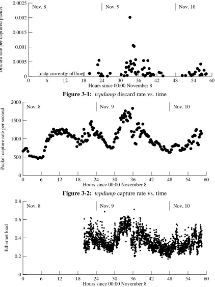
Since we had 10 Mbit/sec (or faster) connections to the Internet via both AlterNet and BAR-RNet, a 10 Mbit/sec Ethernet LAN, and a router rated to run at full Ethernet rates, we did a crude calculation that convinced us that our local network infrastructure could handle the load. (Al-though we had a ‘‘Sniffer’’ monitoring the LAN, we neglected to log network utilization rates at regular intervals; spot checks showed one-second load averages peaking at about 70%, and long-term averages around 30%. See figure 3-3 for an approximation of the load averages.)

(it happened during lunch), we switched to a T3 wired connection, which eliminated the packet losses. We also constructed, but did not have to employ, a low-speed serial line connection to the Teale Data Center, for use in retrieving updated returns if the normal Internet path from Teale became congested by client traffic.

3.2. Server hardware

With sufficiently high-performance and redundant network connections in place, we turned our attention to the server systems. We used one three-processor and two dual-processor Digital 2100 model A500MP server machines; each processor was a Digital Alpha CPU rated at 110 SPECint92. Each dual-processor system was rated at 6,178 SPECrate_int92. The three-processor system had 512 MB of RAM; the dual-three-processor systems each had 256 MB. We maintained an identical copy of the server contents on the disks of each of the three server machines.

Since we wanted to expose only a single top-level URL, and hence a single host name, to clients, we used the Domain Name System (DNS) [13] CNAME mechanism to create a

three-valued binding from www.election.ca.gov to the actual names of the three server hosts.

We hoped that since modern DNS servers randomize the order in which they return the three bindings, clients would end up evenly balanced among the servers. Our experiences partially bore out this expectation; see section 4.3.

The use of several systems, instead of one large one, not only provided cost-effective perfor-mance scaling, it also provided a natural ‘‘warm spare’’ redundancy mechanism. We kept a fourth, somewhat slower, system running at all times, with its own copy of the database. If one of the main servers had failed, we would have rebooted the backup system after changing its IP address to match that of the failed system. We chose not to try to rebind the CNAME to the normal name (and address) of the backup system, since we had no idea how long it would take to propagate this change through the caches in the DNS.

3.3. Server software

The server machines ran DEC OSF/1 V3.0, which supports symmetric multiprocessing and

thus made effective use of the dual processors. We used the NCSA httpd version 1.3 HTTP

server, mostly because we had had extensive experience with this code and believed it could be trusted. However, we soon realized that this software might not support our estimated perfor-mance target, so I modified it slightly to avoid some inefficiencies.

It took me a while to locate the bug and prepare a fix, and anecdotal reports suggest that many potential users who tried the service during this period became frustrated and never came back. We suspect that we would have seen a much higher peak rate in the hours after the polls closed, had this bug not been present.

3.4. Log and trace collection

HTTP servers typically log some information about each request, but the original NCSA serv-er does not log quite enough information to fully investigate the pserv-erformance issues. In par-ticular, it does not log connection duration, and it uses timestamps with 1-second resolution. I modified the server to record more extensive log information about each request, including con-nection duration, CPU time usage, and the number of actual disk reads done for each request. All timing information was done with approximately 1 msec resolution.

At fifteen minute intervals, we collected system-wide statistics on each server machine. These include system load averages, network interface statistics, a snapshot of the protocol control block (PCB) table, network buffer statistics, virtual memory statistics, and disk I/O statistics. (The disk I/O statistics, alas, proved useless because of a minor bug in the particular operating system release running on the servers, but we believe the file system cache was large enough to avoid almost all disk I/O.) We had intended to collect network and transport level statistics

(using netstat -s), but neglected to do until approximately noon on the day after the

elec-tion.

We also set up a workstation running the tcpdump program, to capture all of the traffic on the Ethernet. These traces covered all of November 8 (election day) and November 9, and most of the morning of November 10. We used tcpdump to capture the first 68 bytes of every packet, as well as the total packet length and a timestamp with microsecond resolution. Each set of one million packets was saved, without analysis, to a disk file and then compressed, yielding in-dividual trace files of about 44 Mbytes. We ultimately traced about 209 million packet headers, requiring about 9 Gbytes of storage after compression; some of this data had to be stored off-line, since we only had 6 Gb of spare disk space.

Promiscuous-mode passive monitoring, as done by tcpdump, has the advantage that it does not perturb the network being monitored, but one risks losing some packets because the monitor is overloaded. Fortunately, our monitor system (a DECstation 3000/400) was usually able to keep up. The software gave us an exact count of the number of dropped packets, which revealed a mean lost-packet rate of 0.011%. The peak lost-packet rate was 2012 per million packets, or 2%. (Figure 3-1 shows the actual discard rates, per million-packet set.) We may also have lost a few packets each time a new instance of tcpdump was started.

Figure 3-2 shows the packet capture rates over time; each sample is averaged over one million packets, so the peak rates were much higher. The peak capture rate reached one million packets in 545 seconds, a mean rate of about 1830 packets per second.

0 6 12 18 24 30 36 42 48 54 60 Hours since 00:00 November 8

0 0.0025

0.0005 0.001 0.0015 0.002

Discard rate per captured packet

[data currently offline]

Nov. 8 Nov. 9 Nov. 10

Figure 3-1: tcpdump discard rate vs. time

0 6 12 18 24 30 36 42 48 54 60

Hours since 00:00 November 8 0

2000

500 1000 1500

Packet capture rate per second

Nov. 8 Nov. 9 Nov. 10

Figure 3-2: tcpdump capture rate vs. time

0 6 12 18 24 30 36 42 48 54 60

Hours since 00:00 November 8 0

0.8

0.2 0.4 0.6

Ethernet load

Nov. 8 Nov. 9 Nov. 10

Figure 3-3: Lower bounds on Ethernet load average

4. Overall server statistics

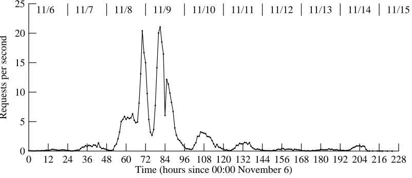
The most basic measure of server load is the rate at which clients issue requests. Figure 4-1 shows the hourly mean request rate (in requests per second) for about nine days around the time of the election. The dip at about noon on November 9 (hour 84) reflects the rain-induced net-work failure. Other dips reflect the wee hours of the morning, suggesting that most of our users were in or near our time zone.

0 12 24 36 48 60 72 84 96 108 120 132 144 156 168 180 192 204 216 228 Time (hours since 00:00 November 6)

0 25

5 10 15 20

Requests per second

11/6 11/7 11/8 11/9 11/10 11/11 11/12 11/13 11/14 11/15

Figure 4-1: Request rates for all servers, average over 1-hour intervals

Peak request rates, over short time scales, far exceeded the hourly means. Figures 4-2 and 4-3 respectively show the peak 1-second and 1-minute rates for each hour. (Note that these rates reflect the times at which connections completed, not at which they were initiated.)

0 12 24 36 48 60 72 84 96 108 120 132 144 156 168 180 192 204 216 228 For hour ending (hours since 00:00 Nov. 6)

0 2000

500 1000 1500

Peak requests per minute

11/6 11/7 11/8 11/9 11/10 11/11 11/12 11/13 11/14 11/15

Figure 4-2: Peak one-minute request rate for all servers, reported hourly

0 12 24 36 48 60 72 84 96 108 120 132 144 156 168 180 192 204 216 228 For hour ending (hours since 00:00 Nov. 6)

0 60

10 20 30 40 50

Peak requests per second

11/6 11/7 11/8 11/10 11/11 11/12 11/13 11/14 11/15

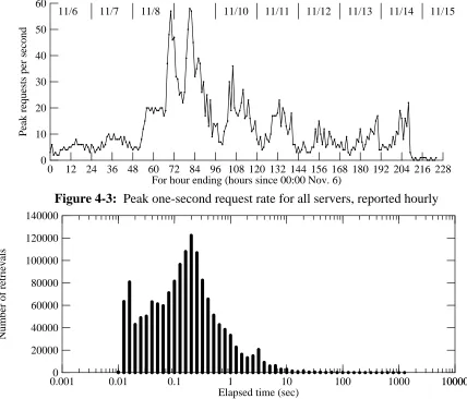
Figure 4-3: Peak one-second request rate for all servers, reported hourly

0.001 10000

Elapsed time (sec)

0.01 0.1 1 10 100 1000 10000

0 140000

20000 40000 60000 80000 100000 120000

Number of retrievals

Figure 4-4: Distribution of connection durations

Figure 4-5 shows the distribution of the sizes, in bytes, of the files retrieved from the servers. (This does not include the considerable overhead data returned in an HTTP response.) Many retrievals fell into a narrow range of sizes under 100 bytes; these were all GIF-format images representing bars in the bar-graph pages. The mean retrieval size was 2394 bytes; the median was 958 bytes. (Ignoring 83406 zero-length retrievals, which are basically client cache valida-tions, the mean was 2535 bytes and the median was 1025 bytes.)

10 100 1000 10000 100000 1e+06 0

400000

100000 200000 300000

Count of retrievals

+85253 zero-length retrievals

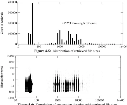
Figure 4-5: Distribution of retrieved file sizes

10 100 1000 10000 100000 1e+06

0.001 10000

Elapsed time (sec)

0.01 0.1 1 10 100 1000 10000

Figure 4-6: Correlation of connection duration with retrieved file size

4.1. Server resource usage

In addition to CPU time, an HTTP server uses several different kinds of system resources, including processes, TCP connections, TCP buffers, and file system buffers. These are all al-located from main memory. Although our server systems had more than enough RAM, we won-dered just how much was necessary. That is, how did the servers make use of their memory resources?

We first looked at the number of entries in the protocol control block (PCB) table. Each TCP connection takes up an entry in this table. One would think that the table size should be ap-proximately the number of active connections, but this is not so.

The TCP protocol specification [15] requires the host that closes a connection to remain in the TIME_WAIT state for a period of twice the maximum segment lifetime (2*MSL). This prevents a subsequent connection from accepting delayed duplicate packets from the closed connection. Since MSL should be two minutes, 2*MSL should be four minutes; however, DEC OSF/1 fol-lows 4.3BSD practice and uses a one-minute timeout here.

state for a few seconds, and then persists in the table in the TIME_WAIT state for quite a while longer. Hence, the number of TIME_WAIT entries can be far greater than the number of ES-TABLISHED connections.

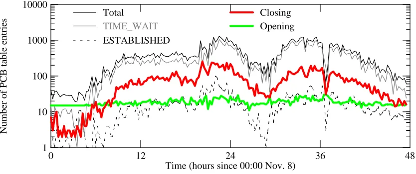
We recorded the contents of the PCB table every 15 minutes. Figure 4-7 shows how the breakdown by state varied over time, for all three servers taken together. (‘‘Opening’’ includes LISTEN, SYN_RCVD, and SYN_SENT; ‘‘Closing’’ includes CLOSE_WAIT, CLOSING, FIN_WAIT_1, FIN_WAIT_2, and LAST_ACK.) Note that nearly all of the table entries are for TIME_WAIT, and most of the rest are ‘‘Closing’’ states. Relatively few of the PCB table entries are used for actual live connections.

0 12 24 36 48

Time (hours since 00:00 Nov. 8) 1

10000

Number of PCB table entries

10 100 1000

Total

TIME_WAIT ESTABLISHED

Opening Closing

Figure 4-7: PCB Table statistics by TCP state

For all servers together, we recorded a peak PCB table size of 1297 entries. The peak number of TIME_WAIT entries was 1049, while the peak number of ESTABLISHED entries was 100. (The actual peaks might have been higher, since we sampled rather infrequently.) Note that if the operating system had used a four-minute timeout for the TIME_WAIT entries, this would have approximately quadrupled the number of these entries.

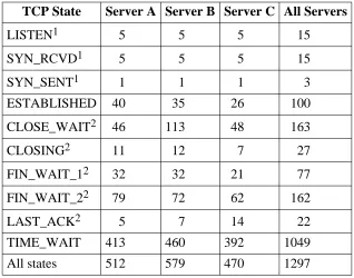
Table 4-1 shows the peak number of entries in each TCP state, as sampled at 15 minute inter-vals. The actual peaks may have occurred between samples. The table shows the peaks for each of the three servers, and for all three servers taken together (within the synchronization error of the sampling process). The latter may be smaller than the sum for all three servers, since the per-server peaks do not always coincide. The states, except for ESTABLISHED and TIME_WAIT, are categorized as ‘‘opening’’ or ‘‘closing’’ transient states, corresponding to the curves in figure 4-7.

The count of LISTEN states includes four other servers besides the HTTP server; the total number of HTTP listeners was always one per machine.

TCP State Server A Server B Server C All Servers

1

LISTEN 5 5 5 15

1

SYN_RCVD 5 5 5 15

1

SYN_SENT 1 1 1 3

ESTABLISHED 40 35 26 100

2

CLOSE_WAIT 46 113 48 163

2

CLOSING 11 12 7 27

2

FIN_WAIT_1 32 32 21 77

2

FIN_WAIT_2 79 72 62 162

2

LAST_ACK 5 7 14 22

TIME_WAIT 413 460 392 1049

All states 512 579 470 1297

Note 1: Connection is ‘‘opening’’ Note 2: Connection is ‘‘closing’’

Table 4-1: Peak counts of PCB table entries by TCP state

reflected as sharp dip in many of the graphs in this paper (for example, see figure 4-7, near hour 36).

Other sites have reported numerous connections stuck in the LAST_ACK state, probably be-cause dialup clients became disconnected from the Internet before the server finished transmit-ting all of its buffered data. We found a few such connections, but never had a significant num-ber at any one time. We also had a small numnum-ber of connections stuck, some for periods of many hours, in FIN_WAIT_1, or less often in FIN_WAIT_2 (these were never more than a small fraction of the total).

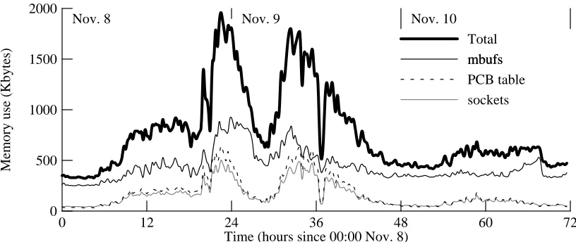
The primary significance of these stuck connections (LAST_ACK and FIN_WAIT_*) is not that they take up PCB table space, but rather that they tie up buffer space for data that has been transmitted but not acknowledged. Over time, an HTTP server could lose significant amounts of kernel memory. This may require using a ‘‘keep alive’’ timer to garbage-collect such connec-tions. How much memory did this table space require? Our logs also recorded memory-usage profiles every 15 minutes; figure 4-8 shows the results for three categories: ‘‘mbufs’’, used mostly to buffer packet headers and data; PCB table entries; and ‘‘sockets’’, used by the kernel to describe active connections. About half of the total use comes from mbufs; PCB table entries and sockets split the rest. In no case (that we sampled) did the total exceed 2 Mbytes, nor did the PCB table size ever exceed about 700 Kbytes. Therefore, we do not believe that even a very busy HTTP server requires much main memory.

0 12 24 36 48 60 72 Time (hours since 00:00 Nov. 8)

0 2000

500 1000 1500

Memory use (Kbytes)

mbufs mbufs

sockets PCB table Total

Nov. 8 Nov. 9 Nov. 10

Figure 4-8: Memory used for network data structures and buffers

McKenney and Dove [11] have pointed out that the use of a linear list for this table can lead to poor performance, and suggest using a hash table for systems with large numbers of active con-nections. They point out that the use of small caches in front of a linear list do not work well in such applications.

In the case of an HTTP server, however, the number of active connections is small. Naive use of McKenney and Dove’s hash-table structure would fill up with useless TIME_WAIT entries (these will almost never be the target of a lookup), slowing lookups and increasing the cost of table insertion and deletion.

A better solution might be to keep the TIME_WAIT entries in a separate structure, such as a queue (since entries will be removed in FIFO order). ‘‘Useful’’ PCB table entries could be kept in a hash-table structure. However, this may not be necessary for an HTTP server. I used the

tcpdump traces to simulate N-entry LRU caches, and found reasonably good hit rates for small

caches. These simulations were done using a tcpdump trace containing 127,367 packets arriving for the servers. This represents approximately 11 minutes starting at 9:40 AM on November 9, one of the peak load periods. Approximately 19198 connections were active during this interval, so these simulated caches warmed up rapidly.

Figure 4-9 shows the simulated hit rates for each individual server (dotted lines) and for all three servers taken as a single entity (solid line). For any individual server, a 16-entry cache would hit almost 80% of the time. If one server was handling the entire load, it would need a 64-entry cache to get an 80% hit rate. One could also look at these results as confirming that a moderately-sized hash table (containing entries only for active connections) would satisfy lookups in one or two comparisons.

4.2. Relative popularity of content files

Our logs contain the name of each file (or map hit) requested, which provides a breakdown of retrievals by file format. It also allows a division into static and dynamic content pages.

0 10 20 30 40 50 60 70 Number of cache entries

0 1

0.2 0.4 0.6 0.8

Cache hit ratio

Individual servers All servers

Figure 4-9: Simulated hit rates for small PCB lookup caches

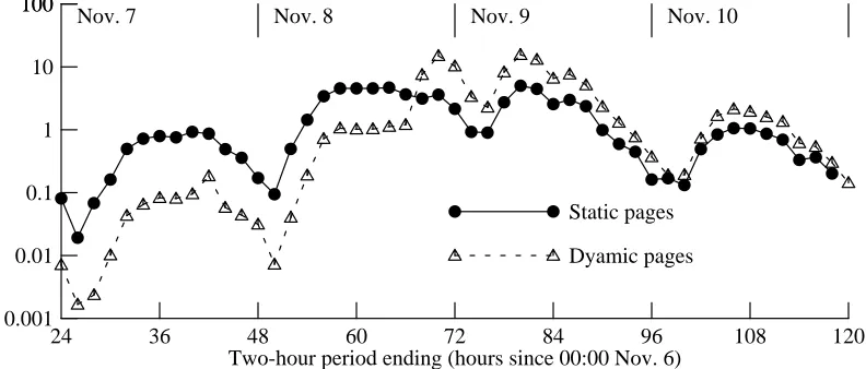
retrievals (by an order of magnitude) were for static pages. After the polls closed (hour 60), dynamic pages led by a large margin, although not a factor of ten.

24 36 48 60 72 84 96 108 120

Two-hour period ending (hours since 00:00 Nov. 6) 0.001

100

Mean requests per second 0.01

0.1 1 10 100

Dyamic pages Static pages

Nov. 7 Nov. 8 Nov. 9 Nov. 10

Figure 4-10: Relative popularity of static and dynamic pages

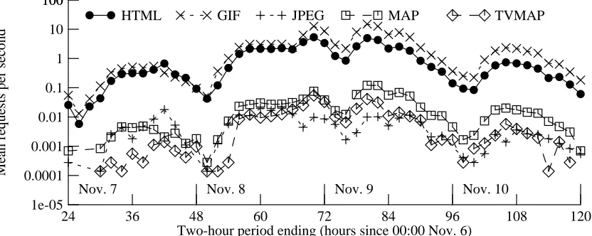
Figure 4-11 breaks down the mean retrieval rate (again, measured over two-hour periods) by file format. GIF and HTML files dominated all others by several orders of magnitude, with GIF files taking the lead after the polls closed (most of these were bar-graph elements).

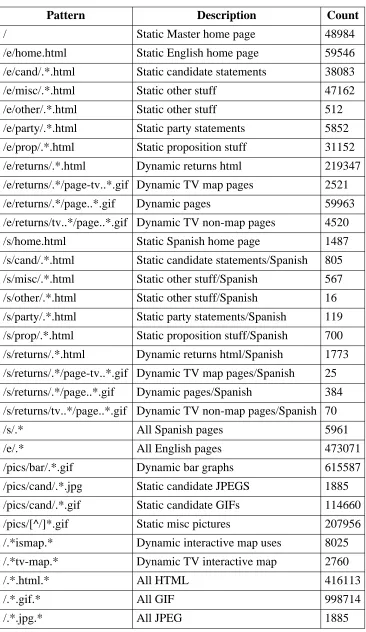
Table 4-2 breaks down the retrievals by various different file name patterns. About 70% of the retrievals were GIF files. 62% of these were bar-graph elements; 11% were candidate photos; 6% were dynamically-constructed images such as maps of voting by counting; the remaining 21% were various static images such as banners, logos, and maps.

24 36 48 60 72 84 96 108 120 Two-hour period ending (hours since 00:00 Nov. 6)

1e-05 100

Mean requests per second _0.0001

0.001 0.01 0.1 1 10 100

HTML GIF JPEG MAP TVMAP

Nov. 7 Nov. 8 Nov. 9 Nov. 10

Figure 4-11: Relative popularity of different file formats

Only 1.3% of the HTML retrievals were for Spanish-language pages, although this may still represent several hundred users. We also had relatively few users of the pages formatted for television broadcast, although we do know that several cable channels used these extensively. Many users retrieved dynamically-constructed maps showing the breakdown of voting by county. Somewhat less often, a user clicked on one of these maps to see additional detail for a given county.

4.3. DNS-based load balancing effectiveness

In section 3.2 I described how we tried to use the Domain Name System (DNS) to spread out the request load among the three server machines. We knew that this would not work perfectly, since there are many caches in the DNS and these tend to reduce short-term randomness.

Over very long periods, the loads did nearly balance. Over the course of an entire day, the total number of requests handled varied among the servers by less than 10%. Figure 4-12 shows the mean hourly loads for each of the three servers, for election day and the day after; at this time scale, the loads are not entirely balanced, but generally are not far off.

At shorter time scales, however, the DNS-based load balancing clearly does not spread re-quests evenly. For example, figure 4-13 shows the per-second request rates for each of the three servers (denoted by different symbols) for one of the busiest minutes. The mean rate, over all three servers, is shown with a solid line. One can see that quite often, one of the servers carries far more than 1/3 of the total request rate. The total load varies enough from second to second to explain most of the inter-server variation; over the course of this minute, no server is obviously favored.

Pattern Description Count

/ Static Master home page 48984

/e/home.html Static English home page 59546

/e/cand/.*.html Static candidate statements 38083

/e/misc/.*.html Static other stuff 47162

/e/other/.*.html Static other stuff 512

/e/party/.*.html Static party statements 5852

/e/prop/.*.html Static proposition stuff 31152

/e/returns/.*.html Dynamic returns html 219347

/e/returns/.*/page-tv..*.gif Dynamic TV map pages 2521

/e/returns/.*/page..*.gif Dynamic pages 59963

/e/returns/tv..*/page..*.gif Dynamic TV non-map pages 4520

/s/home.html Static Spanish home page 1487

/s/cand/.*.html Static candidate statements/Spanish 805

/s/misc/.*.html Static other stuff/Spanish 567

/s/other/.*.html Static other stuff/Spanish 16

/s/party/.*.html Static party statements/Spanish 119

/s/prop/.*.html Static proposition stuff/Spanish 700

/s/returns/.*.html Dynamic returns html/Spanish 1773

/s/returns/.*/page-tv..*.gif Dynamic TV map pages/Spanish 25

/s/returns/.*/page..*.gif Dynamic pages/Spanish 384

/s/returns/tv..*/page..*.gif Dynamic TV non-map pages/Spanish 70

/s/.* All Spanish pages 5961

/e/.* All English pages 473071

/pics/bar/.*.gif Dynamic bar graphs 615587

/pics/cand/.*.jpg Static candidate JPEGS 1885

/pics/cand/.*.gif Static candidate GIFs 114660

/pics/[^/]*.gif Static misc pictures 207956

/.*ismap.* Dynamic interactive map uses 8025

/.*tv-map.* Dynamic TV interactive map 2760

/.*.html.* All HTML 416113

/.*.gif.* All GIF 998714

/.*.jpg.* All JPEG 1885

48 54 60 66 72 78 84 90 96 Time (hours since 00:00 November 6)

0 10

2 4 6 8

Mean requests per second per server

Nov. 8 Nov. 9

Figure 4-12: Mean request rates for each server, showing load balance

0 10 20 30 40 50 60

Seconds 0

30

5 10 15 20 25

Requests per second

For the minute of 09:48, November 9

Figure 4-13: Instantaneous request rates for each server

0.3 0.4 0.5 0.6 0.7 0.8 0.9 1

Busiest server’s fraction of total load 0

100

20 40 60 80

Cumulative percentage of samples

85% worse than 0.39

50% worse than 0.47

25% worse than 0.54 15% worse than 0.58

5% worse than 0.67

Figure 4-14: Cumulative distribution of load imbalances

0.3 0.4 0.5 0.6 0.7 0.8 0.9 1 Busiest server’s fraction of total load

0 100

20 40 60 80

Cumulative percentage of samples

Busiest 1000 1-second periods Busiest 1000 10-second periods Busiest 1000 1-minute periods Busiest 100 5-minute periods Busiest 100 5-minute periods

Figure 4-15: Cumulative distribution of longer-term load imbalances

Our goal in using multiple servers was both to provide redundancy and to improve perfor-mance. Our failure to balance the loads at the shortest time scale suggests that the DNS-based technique cannot provide linear scaling for server performance at peak request rates. Three ser-vers may do better than one server, but probably not three times as well. The clients will most likely see slightly increased response times, not connection failures, since the second-by-second variation in request rate gives a temporarily overloaded server time to catch up.

5. Per-client statistics

How did a typical client use the Election Server? Is there, in fact, a ‘‘typical’’ client? Our logs included client host addresses, so we can analyze the per-client usage patterns. We looked at 1,494,003 retrievals starting on November 6.

Figure 5-1 shows the cumulative distribution of the number of requests per client host. The horizontal axis shows the number of retrievals per client; the vertical axis shows the cumulative number of retrievals. For a given x value, the corresponding y value shows the total number of retrievals done by client hosts that each did x retrievals or fewer.

An especially large number (1083) of hosts made exactly six requests. Analysis of the re-quested file names reveals why: the top-level URL (the only one widely publicized) contains five inlined images. Almost 900 of these six-retrieval hosts fetched all five of these images. 1070 of these hosts (98%) fetched the top-level home page. The remaining hosts were probably running browsers that do not use images (such as Lynx) or with image-retrieval disabled; these clients looked a little deeper into the server.

50% of the requests were done by client hosts that did 155 requests or fewer; 75% were done by clients that did 477 requests or fewer. This suggests that most client hosts were single-user machines (workstations or PCs).

1 100000 Number of retrievals per client

10 100 1000 10000

100 1e+07

Cumulative number of retrievals

1000 10000 100000 1e+06

Figure 5-1: Cumulative distribution of client retrieval count

total. Many of these highly active hosts were actually acting as relays, concentrating requests from many different users. For example, the most-active host is a relay for a California-based company.

Others were time-shared machines. Seventeen individual hosts in this category shared one IP subnet, together accounting for 25982 requests, and should probably be treated as a single large timesharing system.

The scatter plots in figures 5-2 and 5-3 show the peak request rates for each of these 90 most-active hosts. The horizontal position of each mark shows the total number of requests made by the host; the vertical position shows the peak request rate. Figure 5-2 shows the 1-second peak rates; figure 5-3 shows the 1-minute and 1-hour peak. The marks enclosed by a diamond reflect the aggregate behavior of the 17-host cluster.

1000 100000

Number of requests per client host address 10000

1 100

Peak request rate per second

10

Figure 5-2: Short-term peak request rates for most active hosts

Can we tell if these hosts are single-user systems, timesharing systems, or relays? The similarity in peak request rate between the 17-host timesharing cluster and the most-active host, which is a relay, suggests that this may be difficult. (However, see section 7.3.)

1000 100000 Number of requests per client host address

10000 10

10000

Peak request rate per interval

100 1000

1-min intervals 1-hr intervals

Figure 5-3: Long-term peak request rates for most active hosts

indeed a single-user host. Figure 5-4 shows what happened during this burst. In this figure, the horizontal axis shows time passing; each integral position on the vertical axis corresponds to a unique URL. The lines plotted show the starting and ending times for retrieving a giving URL; fat lines correspond to HTML files.

The first URL retrieved in this timeline shows up as a long thin line; this is a moderately large GIF image showing a map of California. The user evidentally clicked on a county, because the next URL is an HTML file giving the returns for a county. The rest of the URLs, all small GIF files, are the bar-graph images for these returns. (The graphing program assigns URL identifiers in order of request completion, not request starting time, and so the left-hand edge of the result-ing curve is ragged.)

4 6 8 10 12

Relative time (seconds) 0

70

10 20 30 40 50 60

URL identifier

Figure 5-4: Timeline for peak-rate burst from a single client

We believe that this client was running the Netscape browser, since careful examination of figure 5-4 shows that GIF retrievals occurred in bursts of about four simultaneous requests; this is precisely the distinctive scheme that Netscape uses to improve perceived latency. The user, who has apparently reached the HTML pages by clicking on county maps, has had to hit the browser’s ‘‘Reload’’ button to get fresh copies of these pages. In Netscape, ‘‘Reload’’ causes retrieval of all inlined images in addition to the HTML file. (Mosaic, on the other hand, only reloads the HTML file.)

0 50 100 150 200 250 300

Reload time (seconds) 0

80

20 40 60

URL identifier

Figure 5-5: Timeline showing lack of effective image caching

This particular client occasionally retrieved the same GIF file several times within the space of a few seconds. Figure 5-6 shows five retrievals of one GIF file, all within less than three seconds. This may be a shortcoming of Netscape’s simultaneous-connection implementation.

0 1 2 3 4 5 6

Relative time (seconds) 0

8

1 2 3 4 5 6 7

URL identifier

Figure 5-6: Timeline showing short-term redundant requests

0 5 10 15 20 25 30 33 Relative time (minutes)

0 30

5 10 15 20 25

URL identifier

Figure 5-7: Timeline showing lack of any client caching

Suppose the busy clients had perfect caches for the GIF files, static HTML files, and version-numbered dynamic HTML files; how much would this have reduced the server load? (This is not completely infeasible; uncachable files could be marked by the server with a time-to-live of zero.) Figure 5-8 shows, for the 90 most active hosts, how many retrievals would they have been made had they been using a perfect cache. Apparently, they would have made almost an order of magnitude fewer requests. Of the 266176 requests made by these hosts, only 62159 (23%) were strictly necessary.

1000 100000

Actual number of requests by host 10000

100 10000

Requests if perfect cache

1000

Figure 5-8: Potential effects of perfect caching

Clients that made fewer requests would not have benefited as much from perfect caching, be-cause they did not do as many redundant retrievals. For example, eleven hosts made 155 re-quests each (the middle of the cumulative distribution in figure 5-1). With perfect caching, they would have made between 56 and 133 requests, with a mean of 103 (66% of the actual number).

6. Network path statistics

We were interested in the nature and behavior of the paths taken through the Internet between our clients and our servers. We did two kinds of path measurements: post-election measure-ments of paths to a large subset of the actual clients, and periodic probes during the election to our servers from a few selected sites.

6.1. Post-election path measurements

In an attempt to characterize the actual paths between our servers and their actual clients, I started by extracting 19,070 host addresses from the server logs. This covers the 1,328,862 re-quests made between 00:00 November 6 and 14:00 November 10.

I then generated scripts that probed the path to each of these hosts. For each host, I ran

traceroute and two sets of of ping trials. Traceroute attempts to discover the sequence of routers

taken to reach a destination, and also measures the delay to each router and the final destination. However, traceroute uses an indirect mechanism and does not always yield a full path; it can also be confused by shifting paths. Ping simply sends a series of ICMP Echo [16] packets to the destination, and measures the time until the corresponding ICMP Echo Reply packets come back. I used ping to make ten measurements to each destination with each of two packet sizes, 56 bytes and 536 bytes.

Network round-trip time and timeouts (for non-responsive hosts) limit the speed at which these probes can be done. Even though I ran 26 probes in parallel, it took from 18:21 on Novem-ber 10 to 13:43 on NovemNovem-ber 16 to collect the results. Clearly, over this period the path charac-teristics could have changed quite significantly, especially on paths subject to occasional over-load. And since these probes were made after the load on the election servers had declined significantly from its peak, the network state during the probing could have been quite different from its state during the peak election load. However, we did not want to complicate things by doing the path-probing during the period of peak load.

Another consequence of doing the probes several days after the peak load is that many of the IP addresses failed to respond to any probes. I only received ping responses from 52% of the hosts, and complete traceroute paths from 44%. (43% gave us both kinds of information). Non-responsive host addresses might be behind firewalls, or might have been connected by dialups, or might have been dynamically assigned for brief durations.

6.1.1. Traceroute results

0 5 10 15 20 25 30 Path length in hops

0 1000

200 400 600 800

Number of hosts

Figure 6-1: Distribution of path lengths to clients

0 5 10 15 20 25 30

Path length in hops 0

100000

20000 40000 60000 80000

Number of retrievals

Figure 6-2: Weighted distribution of path lengths to clients

6.1.2. Ping results

Of the hosts that responded at least once to an ICMP Echo packet, the average host replied to about 9.5 of the 10 Echos sent in each trial. For the 9840 hosts responding to 56-byte pings, the mean round-trip time was 207 msec; weighted by the number of retrievals the mean was 146 msec. That is, clients with lower delays tended to make more requests. For the 9755 hosts responding to 536-byte pings, the mean delay was 322 msec, and the weighted mean delay was 229 msec.

Figure 6-3 shows the distribution of round-trip times for both packet sizes. 56-byte data are marked with filled circles; 536-byte data are marked with open squares. Note that the distribu-tions are trimodal; the 56-byte values peak near 10 msec, 80 msec, and 600 msec. The 536-byte values peak near 25 msec, 100 msec, and 600 msec.

1 100000 Round-trip time in msec

10 100 1000 10000

0 1200

200 400 600 800 1000

Number of hosts

56 bytes

536 bytes

Figure 6-3: Distribution of round-trip times

1000 1e+08

Inferred bandwidth (bits/sec)

10000 100000 1e+06 1e+07

1 10000

Number of hosts

10 100 1000

Ethernet T1

56 K 14.4 K

Figure 6-4: Distribution of inferred bandwidths

Figure 6-4 shows several distinct features. The bandwidth estimates above 10 Mbit/sec are clearly bogus, since they are certainly the result of noise in the measurements; all paths included at least one hop on a 10 Mbit/sec Ethernet. None of the delays were below 6 Kbit/sec, suggest-ing that relatively few of the hosts that responded to probes were on low-speed dialups. The distribution shows several peaks, one at approximately 15 Kbit/sec, a broad peak around 200 Kbit/sec, a sharp peak at 400 Kbit/sec, and a broad one between 3 Mbit/sec and 5 Mbit/sec. This distribution suggests that a large portion of the client hosts are well-connected to the Internet, via fractional T1, full-speed T1, or faster links. However, since only about half of the clients responded to post-election pings, low-speed (dialup) hosts probably represent a much larger frac-tion than this distribufrac-tion indicates.

0 5 10 15 20 25 30 Hop count

100 1e+07

Inferred bandwidth (bits/sec)

1000 10000 100000 1e+06

Figure 6-5: Correlation between hop count and estimated bandwidth

6.2. Periodic probes during the election

For a period of about two days (November 8 and 9), we ran periodic probes to our servers

from three sites on the Internet: Software Tool & Die in Massachusetts (world.std.com),

Marquette University in Wisconsin (marque.mscs.mu.edu), and the University of

Pennsyl-vania (upenn.edu). Every 15 minutes, the probe scripts ran ping to our server to measure the

round-trip time for ICMP Echos of several different sizes, and ran a simple test program to measure the retrieval time for several pages from the server. One page was a 3KB HTML file; the other was a 7KB GIF file.

The probe scripts also used traceroute to discover the path taken between the probe sites and

our server. The path from upenn.edu consistently took 15 hops. The path from

marque.mscs.mu.edu varied continually, between 16 and 18 hops. The path from

world.std.comstarted at 6 hops, but shifted to a 9-hop path late on the evening of November 9.

The top graph in figure 6-6 shows how the sampled round-trip time values varied over time (these measurements are for minimal-sized ICMP Echos). Note that the horizontal axis shows Eastern Standard Time, not Pacific Time. Filled circles show data from

marque.mscs.mu.edu; plusses show data from upenn.edu; open squares show data from

world.std.com. The RTTs increase slightly during the periods of heavy load on our server. The bottom graph in figure 6-6 shows the cumulative distribution of round-trip time samples.

The top graph in figure 6-7 shows how retrieval times for the HTML file varied over time. The bottom graph shows the cumulative distribution. The time axis in each of these graphs is on a log scale, because in a few cases, retrievals took many minutes. This probably reflects episodes of heavy packet loss somewhere in the network, or perhaps a temporary loss of network connectivity. Retrieval times in the range of one to ten seconds were distressingly common, suggesting that users might not have always been pleased with response time. However, most of the retrievals did take less than one second.

0 12 24 36 48 Time (hours since 00:00 Nov 8) EST

50 250

100 150 200

Round-trip time (msec)

Nov. 8 Nov. 9

50 100 150 200 250

Round-trip time (msec) 0

1

0.2 0.4 0.6 0.8

Cumulative fraction of probes

marque.mscs.edu upenn.edu world.std.com

Figure 6-6: Sampled round-trip times from periodic probes

Note that this method may not adequately reflect network congestion, since it measured RTTs for single packets. A packet-pair approach [3] would have been more appropriate.

7. Interarrival patterns

Several recent studies [8, 10, 14] have suggested that packet interarrival times tend to fit dis-tributions other than Poisson. Does the data from our traces confirm this?

Using the server logs (with 1-msec timestamp resolution) and the tcpdump traces (with 1-usec resolution), I was able to obtain interarrival distributions for several categories of events. These distributions support the observations by others that real networks with real users cannot be modelled by a Poisson process.

7.1. Packet arrivals

Because of the immense volume of the tcpdump traces, I concentrated on the data for just the

2

busiest date, November 9 . I looked at the arrivals of several different classes of packets, for the

0 12 24 36 48 Time (hours since 00:00 Nov 8 EST)

100 1e+06

Round-trip time (msec) for home.html

1000 10000 100000

Nov. 8 Nov. 9

100 1e+06

Round-trip time (msec) for home.html

1000 10000 100000

0 1

0.2 0.4 0.6 0.8

Cumulative fraction of probes

marque.mscs.edu upenn.edu world.std.com

Figure 6-7: Sampled HTML retrieval times from periodic probes

three server hosts. These classes include: all incoming HTTP packets, all outgoing HTTP pack-ets, all incoming HTTP packets with the TCP SYN bit set (representing a connection request), and all outgoing HTTP packets with the SYN bit set (representing acceptance of a connection request). (Although the traces only show that the incoming packets appeared on the LAN, prior experience suggests that nearly all of these packets were in fact received by the server kernels, although they may have then been discarded due to resource limits.)

Figure 7-1 shows the cumulative distributions of interarrival times for these four classes. The median of each distribution is marked on the curve; the mean interarrival time is shown in the key. The thick gray line shows a Poisson distribution with the same mean interarrival time as the ‘‘all incoming HTTP packets’’ curve (13 msec); it has a much different shape than the actual data.

Figure 7-2 shows the same distributions, but for a particularly busy 1-minute period. Again, the Poisson distribution with the same mean rate as the ‘‘all arriving HTTP packets’’ curve is shown by a thick gray line. Observe that these curves generally have the same shape as those for the full 24-hour period, even though the mean rates are higher.

0 12 24 36 48 Time (hours since 00:00 Nov 8 EST)

100000 800000

200000 300000 400000 500000 600000 700000

Inferred bandwidth (bits/sec)

Nov. 8 Nov. 9

0 200000 400000 600000 800000 1e+06

Inferred bandwidth (bits/sec) 0

1

0.2 0.4 0.6 0.8

Cumulative fraction of probes

marque.mscs.edu upenn.edu world.std.com

Figure 6-8: Network bandwidths inferred from periodic probes

0.01 100000

Interarrival time in msec

0.1 1 10 100 1000 10000 100000

1000 1e+07

Cumulative number of events

10000 100000 1e+06

All incoming, mean 13 ms 4.9 msec

Outgoing SYNs, mean 113 ms 44 msec

Incoming SYNs, mean 100 ms 40 msec

All outgoing, mean 14 ms 2.7 msec

Poisson for ’All incoming’

Figure 7-1: Cumulative distributions of interarrival times, Nov. 9

Figure 7-4 shows the same distributions, but for the busy 1-minute period. In this graph, we can see that the Poisson curve is a fairly good fit for the incoming packet arrivals, although it tends to underpredict the number of very short and very long interarrival times.

0.01 1000 Interarrival time in msec

0.1 1 10 100 1000

10 100000

Cumulative number of events

100 1000 10000

All incoming 2.4 msec

Outgoing SYNs 22 msec

Incoming SYNs 17 msec

All outgoing 1.8 msec

Figure 7-2: Cumulative distributions of interarrival times, Nov. 9 09:48

0.01 10000

Interarrival time in msec

0.1 1 10 100 1000 10000

100 1e+06

Number of events ₁₀₀₀

10000

100000 All incoming

Outgoing SYNs Incoming SYNs All outgoing

Figure 7-3: Distributions of packet interarrival times, Nov. 9 (same data as figure 7-1)

0.01 1000

Interarrival time in msec

0.1 1 10 100 1000

1 10000

Number of events ₁₀

100 1000

All incoming, mean 4.5 ms Outgoing SYNs, mean 35 ms Incoming SYNs, mean 29 ms All outgoing, mean 4.9 ms

Figure 7-4: Distributions of packet interarrival times, Nov. 9 09:48

The ‘‘all incoming’’ and ‘‘all outgoing’’ distributions also sharply peak at about 120 usec. This may be a reflection of our routing topology: since we had two different routes to the Inter-net, the servers often chose the wrong outbound router. This router would issue an ICMP Redirect to the server, and also retransmit the packet across the Ethernet to the correct router. Thus, numerous outgoing packets appeared twice, but these were mostly short (60-byte) packets since the subsequent longer packets followed the Redirected route.

0 100 200 300 400 500 600 700

Bytes per packet 2e+06

1.4e+07

4e+06 6e+06 8e+06 1e+07 1.2e+07

Cumulative number of packets

Outgoing packets Incoming packets All packets

Figure 7-5: Cumulative distributions of packet sizes, Nov. 9

0 100 200 300 400 500 600

Bytes per packet 10

1e+07

Number of packets

100 1000 10000 100000 1e+06

Circles: outgoing packets; Triangles: incoming packets; Squares: all Election-server packets

Figure 7-6: Distributions of packet sizes, Nov. 9

7.2. Request arrivals

The real distributions tend to follow the Poisson curves for interarrival times below the mean, but have much larger tails. The real data also shows two large peaks, at 1 msec and at about 7 msec. The 1-msec peak is a measurement artifact of the 1-msec timestamp resolution, and cor-responds to the number of events with all interarrival times <= 1 msec. The 7-msec peak prob-ably reflects the CPU-time cost to dispatch a new process for each request; note that the single-server distribution shows almost no interarrival times below about 6 msec. These two distribu-tions imply that at short time-scales, requests arriving at the server hosts do follow a Poisson distribution, but queueing delays in the servers cause the server processes to see a non-Poisson distribution.

0.1 10000

Request interarrival time in msec

1 10 100 1000

1 100000

Number of events

10 100 1000 10000

Actual, all servers Poisson, mean 117 msec

Actual, 1 server

Poisson, mean 355 msec

Figure 7-7: Distributions of request interarrival times, Nov. 9

7.3. Per-client request arrivals

In addition to the overall arrival pattern, I looked at the interarrival time distribution for re-quests from several individual sources mentioned in section 5: the busiest proxy, the 17-host timesharing cluster, and the single-user host with the highest peak request rate. These distribu-tions are shown in figure 7-8, along with Poisson distribudistribu-tions with similar mean interarrival times.

0.1 1e+08

Interarrival time in msec

1 10 100 1000 10000 100000 1e+06 1e+07

1 10000

Number of events ₁₀

100 1000

Bursty client 17-host cluster

Busiest proxy

Poisson, 84 ms Poisson, 1468 ms

Poisson, 1623 ms

Figure 7-9 shows the same data as in figure 7-8, as cumulative distributions.

0.1 10000

Interarrival time in msec

1 10 100 1000

10 100000

Cumulative number of events

100 1000 10000

Bursty client 17-host cluster Busiest proxy

Poisson, mean 84 ms Poisson, mean 1468 ms Poisson, mean 1623 ms

Figure 7-9: Cumulative distributions of request interarrivals, selected clients

Once again, the actual distributions deviate significantly from the Poisson distributions for interarrival times much above the mean, but match fairly closely for smaller values. Also note that the single-user system has a much lower mean than either of the multi-user distributions, and the busy proxy has a much sharper peak than the timesharing cluster. A straightforward proxy server must funnel all requests through a single synchronization bottleneck, causing queueing delays not seen in a timesharing system. This ‘‘signature’’ in the interarrival time distribution may allow one to distinguish proxies from other kinds of clients.

7.4. Summary of arrival data

While we have not yet done extensive analysis at numerous time scales, it does appear that the packet interarrival times we measured do diverge from a pure Poisson process, especially for longer measurement periods, and they show an excess of very short and very long interarrival times. Likewise, HTTP request interarrival rates deviate from Poisson, especially when viewed by the server process itself.

Recent work by others has suggested that network arrival patterns are self-similar rather than Poisson [10], and that the self-similarity arises from the behavior of ‘‘on/off’’ sources [17]. Crovella and Bestavros have shown this specifically for other HTTP traces [5]. One charac-teristic of such sources is a long tail in the interarrival time distribution, such as is seen in figures 7-7 through 7-9.

8. TCP behavior patterns

Because we had extensive tcpdump traces, this provides an opportunity to look at the details of client and server TCP behavior under conditions of heavy server load.

8.1. Packets per connection

I started by counting the number of packets per connection, both received and transmitted (from the point of view of the server). The distribution and cumulative distribution are shown in figure 8-1. The mean number of packets per connection was 17; 8.75 from the client to the server, and 8.26 from the server to the client. For the median connection, the client sent between 6 and 7 packets and the server sent between 5 and 6 packets, with a total of between 12 and 13 packets exchanged. The means are larger than the medians because a few connections trans-ferred hundreds or thousands of packets.

These counts include retransmissions; this increases the number of packets per connection (see section 8.3). The counts also include ‘‘connections’’ that failed to complete; these connections often (but not always) involve just a few packets, which could tend to push the medians down. A successful HTTP transaction seems to involve 9 or 10 TCP packets (although fewer would be possible with more effective piggy-backing of ACKs).

About 6% of the ‘‘connections’’ traced seem to have exchanged too few packets to have been successful. Some or most of these apparently too-short connections might be artifacts of the trace-analysis process, which analyzes each sequence of 1 million packets independently and so may truncate connections that take place near one end of such a sequence. A few others may be artifacts of the trace-collection process, which did occasionally lose packets (see figure 3-1).

1 1000

Packet count per connection

10 100

1 1e+06

Number of connections ₁₀

100 1000 10000

100000 Total packets

Input packets Output packets

1 100000

Packet count per connection

10 100 1000 10000

0 110

20 40 60 80 100

Cumulative per cent of connections

Total packets Input packets Output packets

The relatively small number of packets per connection has several implications:

•Any kernel modifications that speed up the handling of packets for an existing

con-nection ought not to significantly increase the cost of creating and deleting connec-tions.

•Most of these TCP connections will be operating in the ‘‘slow-start’’ regime [7], in

which the sender uses an artificially small window, and so will not be able to obtain full network bandwidth, especially over high-delay paths.

8.2. PCB table search costs

The kernels running on the servers used a linear search of the PCB table, which is known to impose high CPU costs when the table is large (see 4.1); how large is this cost?

Each received TCP packet causes a search for a PCB table entry, and so this search cost is on the critical path for replies to incoming packets. In particular, the speed with which a server responds to a client’s SYN packet depends only on the cost of handling packet headers and doing PCB table operations, not on the costs of handling packet data or synchronizing with application processes. Therefore, I analyzed the tcpdump traces to measure, for each arriving SYN, the time it took one of the server systems to respond. The distribution is shown in figure 8-2.

0.01 100000

Response time in msec

0.1 1 10 100 1000 10000 100000

1 100000

Number of events

10 100 1000 10000

Figure 8-2: Distribution of servers’ response times to SYNs, Nov. 9

The distribution has a sharp peak, at about 800 microseconds. There does not appear to have been many responses that could have been delayed by lengthy table searches; 72% of the responses took under 1 msec, and 97% took under 2 msec; less than 1% took longer than 5 msec. This puts an upper bound of 28% on the number of searches delayed more than 1 msec; since much of the delay could be cause by queueing in the network or in the server, the actual fraction could be much smaller.

connections/second. Experiments with simple test programs suggest that a single-CPU system does indeed bottleneck at about 80 TCP connections per second, even without doing any HTTP processing.

The distribution in figure 8-2 shows that for most of the connections in the trace, the response time was actually quite good. However, the connections that did suffer from poor per-packet response time were probably those in progress during periods of heavy load, when the PCB table size, and thus the excess PCB lookup cost, is greatest. This is precisely the wrong time to im-pose extra costs on connections, since the system’s resources are already stretched. Figure 8-3 shows this correlation between load, PCB table size, and response time.

0 3 6 9 12 15 18 21 24

Time (hours since 00:00 Nov. 9) 0

1800

300 600 900 1200 1500

Total PCB table entries

Median SYN response time (usec) Peak requests per minute

Request rate: peak 1-minute rate over 10-minute intervals PCB table size: sampled at 15-minute intervals

Response time: median response time over 10-minute intervals

Figure 8-3: Correlation between request rate, PCB table size, and response time

8.3. TCP retransmissions

TCP senders retransmit packets when they do not receive an acknowledgement within a timeout interval. The timeout value is a function of the sender’s estimated round-trip time (RTT), following algorithms that have been developed over years of experience and analysis [7, 9].

One can learn several things about the network and its packet sources by observing TCP packet retransmissions in tcpdump traces, and analyzing the retransmission counts and inter-arrival times.

8.3.1. SYN retransmissions