Munich Personal RePEc Archive
An Adaptive Succesive Over-relaxation
Method for Computing the Black-Scholes
Implied Volatility
Li, Minqiang
Gerogia Institute of Technology
21 January 2008
An Adaptive Successive Over-relaxation Method for Computing
the Black-Scholes Implied Volatility
January 21, 2008
A new successive over-relaxation method to compute the Black-Scholes implied volatility is introduced. Properties of the new method are fully analyzed, including global well-definedness, local convergence, as well as global convergence. Quadratic order of convergence is achieved by either a dynamic relaxation or transformation of sequence technique. The method is further enhanced by introducing a rational approximation on initial values. Numerical implementation shows that uniformly in a very large domain, the new method converges to the true implied volatility with very few iterations. Overall, the new method achieves a very good combination of efficiency, accuracy and robustness.
Keywords: Successive over-relaxation, Black-Scholes formula, Implied volatility, Rational ap-proximation.
1. Introduction
A breakthrough in modern financial theory is the Black-Scholes-Merton theory of option pricing, developed by Black and Scholes (1973), Merton (1973, 1976) and many others. In 1997, the Nobel prize in Economics was awarded to Merton and Scholes for the discovery and extension of this theory. As the press releases described it, the Black-Scholes theory is “among the foremost contributions to economic sciences over the last 25 years.” The ultimate result of the theory is the celebrated Black-Scholes formula, which is being used daily by traders around the world nowadays. Besides being used to price options on stocks, the Black-Scholes theory is also used to value options on futures, options on currencies, options on interest rates, etc. Even models that are out of the Black-Scholes framework, such as stochastic volatility models and more recently Levy-process type models, still refer to the Black-Scholes model as the basic benchmark. See, for example, Heston (1993), and Carr and Wu (2003). The use of the Black-Scholes formula is so pervasive that Nigel Goldenfeld, a Physics professor at the University of Illinois at Urbana-Champaign, claims that the Black-Scholes formula is the most frequently used equation by human beings nowadays, beating both Newton’s laws of motion in classical mechanics and Schr¨odinger’s equation in quantum mechanics.
In practice, traders often do not use the Black-Scholes formula to price options. Rather, they observe the actual price on the market and then use the Black-Scholes formula backwards to compute the volatility parameter, called the implied volatility. Early academic development of this concept and on its applications includes Latan´e and Rendleman (1976), and Schmalensee and Trippi (1978). The implied volatility is a useful quantity because it is a succinct way to talk about option prices. In fact, traders are usually more comfortable to talk in terms of implied volatilities than prices themselves. Market participants also pay close attention to the implied volatility since it serves as a forward-looking measure of people’s expectation about future market movements. The Black-Scholes volatility is also a useful concept for models outside the Black-Scholes framework. For example, people are constantly interested in whether a new proposed model can produce the Black-Scholes implied volatility curve observed on the market. The importance of the implied volatility is most evident in the classical NatWest Markets case. In 1997, NatWest lost 90.5 million pounds due to consistent underestimating of implied volatilities it used to price interest rate swaptions.
algorithm might not converge at all to the true implied volatility. The Dekker-Brent algorithm uses a combination of bisection, secant and inverse quadratic interpolation, and is guaranteed to converge. Some commercial software, such as MATLAB, chooses to use the Dekker-Brent algorithm, possibly because of its robustness. However, the Dekker-Brent algorithm is usually slower than the Newton-Raphson algorithm. For example, as Li (2008) reports, the number of inversions one has to do for the S&P 500 index options for the period January 1996 to December 2004 is about 700,000. On a typical computer, to achieve 10−6 accuracy in total volatility (defined as the volatility multiplied by the square root of maturity), it takes the built-in function “blsimpv” built-in MATLAB hours to fbuilt-inish these built-inversions, while the Newton-Raphson algorithm without vectorization takes about 960 seconds.
In this paper, we introduce a new method to compute the Black-Scholes implied volatility based on successive over-relaxation. Thus, our method is an iterative method and not in closed form. We study this method for two reasons. First, although the approximation domain in Li (2008) is fairly large, in practice, total volatility can be well above 1, especially for energy derivatives, or equity derivatives near earnings announcements. Thus, we use a much larger domain in this paper, with moneyness ranging from −3 to 3 and total volatility ranging from 0 to 6. This domain should cover almost all practical applications. Second, we try to search for a method which has the best combination of efficiency, accuracy and robustness. We will see that our method can achieve quadratic order of convergence, the same order as the Newton-Raphson algorithm. On the other hand, our method is robust as is the case for the Dekker-Brent algorithm. With just five iterations our method achieves a uniform error in the total volatility in the order of 10−13 inside the huge domain. The time it takes to invert one million options is about 10 seconds.
Our first contribution in this paper is that we design a new method to compute the implied volatility. The basic idea of our method is to split the Black-Scholes formula into two parts and to search for the implied volatility iteratively. To improve efficiency, we introduce a relaxation parameter. We call our method with over-relaxation the SOR algorithm. Unlike the Newton-Raphson algorithm, the computation of vega is not needed in our method. We analyze the well-definedness, local and global convergence properties of the SOR algorithm in detail. In Theorem3.1, we show that when the relaxation parameter is large enough, theSORalgorithm is always globally well-defined. This is a very attractive feature because it gives rise to robustness of our algorithm. Theorem3.2shows that the local convergence is dictated by the behavior of the iteration function near the true implied volatility. Theorem3.3shows that only two convergence patterns can occur, monotone or oscillating. Theorem3.4and3.5show the convergence patterns of price errors and implied volatility errors, respectively. The most interesting analysis is on global convergence, which is usually very difficult to study. We obtain many interesting results. Theorem3.6 and 3.7 study two important special cases where the moneyness or the relaxation parameter is 0, respectively. Theorem3.8is shows that when the relaxation parameter is larger than some threshold value, the SOR algorithm is always globally convergent. The case where the relaxation parameter is smaller than the threshold value is much harder to analyze and we content ourselves by giving three sufficient conditions on global convergence in Theorem3.9,3.10
and 3.11.
The second contribution of this paper is that we introduce two convergence acceleration tech-niques to the SORalgorithm. The basicSORalgorithm usually has a linear order of convergence, as is shown in Theorem 4.1. The first acceleration technique is based on dynamic relaxation, where we adaptively adjust the relaxation parameter at each iteration. We call this theSOR-DR
technique, where at each iteration step we perform a nonlinear extrapolation, with the weight adaptively adjusted. We call this the SOR-TS algorithm. Theorem 4.4 shows the global well-definedness and convergence properties and local convergence patterns for theSOR-TSalgorithm, while Theorem 4.5shows that it has a quadratic order of convergence.
Our third contribution is on numerical implementation of our algorithms. To further enhance the efficiency of our algorithms, we introduce a rational approximation on the initial estimates, in the same spirit as Li (2008). We show numerically that uniformly in a very large domain, our accelerated algorithms converge to the true implied volatility with very few iterations. We also briefly compare the SOR-TS algorithm with other methods such as the Newton-Raphson algorithm and the Dekker-Brent algorithm, and show that the SOR-TS algorithm achieves the best combination of accuracy, efficiency and robustness.
Finally, we extend our successive over-relaxation method to the computation of implied correlation in the Margrabe formula, the normal implied volatility in the Bachelier formula, and the critical stock price in a compound call on call option. The extension to the Margrabe formula is straightforward. The extensions to the Bachelier implied volatility and critical stock price require some analysis, and Theorem 6.1 and 6.2 show that for both applications, the successive over-relaxation method is globally well-defined and convergent with a quadratic order of convergence. These three examples demonstrate that the idea of successive over-relaxation is not limited to the computation of the Black-Scholes implied volatility, but rather applicable in a much wider range of financial problems.
The rest of the paper is organized as follows. Section2introduces the problem of computing the Black-Scholes implied volatility. Section 3 introduces the basic successive over-relaxation method and studies its well-definedness, local and global convergence properties. Section4 con-siders two acceleration techniques, one based on dynamic relaxation and the other on sequence transformation, and shows that both of them achieve quadratic order of convergence. Section5
implements all three algorithms with a rational approximation enhancement. Section6 demon-strates that the successive over-relaxation method is applicable in many other financial problems through three additional examples. Section7 concludes. Proofs are in the Appendix.
2. The Implied Volatility Problem
Let C be the price of a call option at time twith expiration date T and strike price K. Let S
be the current stock price, σ the volatility of the stock, r the risk-free interest rate, and δ the dividend rate. Then the Black-Scholes formula expresses C in closed form as follows:
C(S, t;r, σ, T, K, δ) =Se−δ(T−t)N(d1)−Ke−r(T−t)N(d2),
where
d1=
log(Se(r−δ)(T−t)/K) σ√T −t +
1 2σ
√
T −t, d2 =d1−σ
√
and N(·) is the cumulative normal distribution function. Let us first define the normalized call option pricec(·,·) by
C(S, t;r, σ, T, K, δ) =Se−δ(T−t)c¡log(Se(r−δ)(T−t)/K), σ√T−t¢.
The function c(x, v) is given by
c(x, v) =N³x v +
v
2 ´
−e−xN³x v −
v
2 ´
, (1)
where the moneynessx and total volatilityv are given by
x= log(Se(r−δ)(T−t)/K), v=σ√T−t. (2)
A call option with x > 0, x = 0 and x < 0 is said to be in-the-money, at-the-money, and out-of-the-money, respectively. Following Li (2008), we call equation (1) the dimensionless Black-Scholes formula.
The dimensionless Black-Scholes formula implicitly gives v as a function of c and x and is the starting point for our successive over-relaxation method. This dimensionless formula clearly states that the Black-Scholes formula is essentially a relation between three dimensionless quantities, namely the normalized price c, the integrated volatility v and the moneyness x. Given observed values of S, t, r, T, K, δ and option price C, we first calculate c according to
c=C/(Se−δ(T−t)) andxaccording to equation (2), and then computevthrough some algorithm. The implied volatilityσ can then be obtained by dividing v by √T−t.
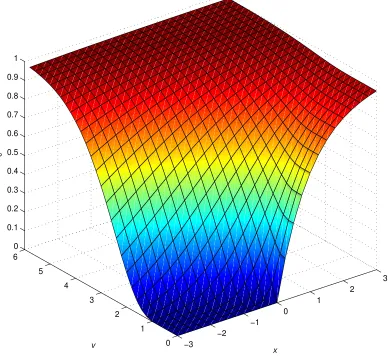
Figure 1 gives a surface plot for the normalized call option pricec when the moneyness x
ranges from−3 to 3, and the volatilityvranges from 0 to 6. As we see, when |x|/v is large,c is very insensitive tovand the inversion is not very meaningful because a tiny change inc(x, v) due to measurement error can give rise to a huge change inv. Thus we will omit these regions in the numerical implementation of our algorithms in Section5 by imposing the restriction|x|/v≤3. We only need to consider inverting call options because by the put-call parity in the Black-Scholes theory (see Stoll 1969), we have C =P +Se−δ(T−t)−Ke−r(T−t). Writing out in
nor-malized call and put prices, we have
c(x, v) =p(x, v) + 1−e−x, (3)
where the normalized put price is defined as the ratio of the actual put priceP and the quantity
Se−δ(T−t). If we are given a put option with moneyness x and normalized put price p, we will simply invert a call option with moneyness x and normalized call pricec=p+ 1−e−x.
Finally, we only need to consider options with moneynessx ≤ 0. This is because we have the following symmetry, which we call the “in-out” duality:
If we need to invert the Black-Scholes formula for an option with moneyness x ≥ 0 and nor-malized call price c, we can as well use the right hand side of the above equation to invert its dual option with moneyness x′ = −x ≤ 0 and normalized call price c′ = exc+ 1−ex. This is also in line with industry practice of treating out-of-the-money options as more informative than in-the-money options. Another rationale to invert out-of-the-money options is the follow-ing. Letting bv be the estimate of the true volatility v∗ that one gets from inverting the dual out-of-the-money option when x >0, then the “in-out” duality gives
|c(−x,bv)−c(−x, v∗)|=ex|c(x,vb)−c(x, v∗)|>|c(x,bv)−c(x, v∗)|.
That is, if we use “in-out” duality to compute the implied volatility for an in-the-money option, the error in terms of price for the in-the-money option is always smaller than that for its dual out-of-the-money options.
3. The Successive Over-relaxation Method
3.1. The SOR algorithm
In this section, we establish a numerical method to compute the implied volatility which is based on the idea of successive over-relaxation. We also analyze the properties of the new method, including global well-definedness, local convergence, as well as global convergence.
We will use n(·) to denote the standard normal density function. The following functions will play important roles, so we give them specific names in order to shorten expressions:
n+(x, v) =n(x/v+v/2), (5)
N+(x, v) =N(x/v+v/2), (6)
N−(x, v) =e−xN(x/v−v/2), (7)
c+(x, v) =N+(x, v) +N−(x, v). (8)
Notice that the dimensionless Black-Scholes formula now becomesc(x, v) =N+(x, v)−N−(x, v). By the discussion in Section 2, we only consider x ≤ 0 and v > 0. The following lemma is very useful later when we analyze the properties of our method. Because of the well-known discontinuity of the Black-Scholes formula, we consider thex <0 and x= 0 cases separately.
Lemma 3.1. When x <0, we have
1) N+(x, v) is strictly increasing in v. Furthermore, N+(x,0+) = 0 and N+(x,+∞) = 1;
2) N−(x, v) is strictly increasing in v for v ≤ p2|x| and decreasing in v for v > p2|x|. Furthermore,N−(x,0+) =N−(x,+∞) = 0;
4) c+(x, v) is strictly increasing in v. Furthermore, c+(x,0+) = 0, and c+(x,+∞) = 1; 5) Let v >0, u >0 andv6=u. Then
u2
2|x|
£
c+(x, v)−c+(x, u)¤< c(x, v)−c(x, u)< v 2
2|x|
£
c+(x, v)−c+(x, u)¤. (9)
When x= 0, we have
1) N+(0, v) is strictly increasing in v. Furthermore, N+(0,0+) = 1/2 and N+(0,+∞) = 1; 2) N−(0, v) is strictly decreasing inv. Furthermore, N−(0,0+) = 1/2 and N−(0,+∞) = 0; 3) c(0, v) is strictly increasing inv, and strictly concave inv. Furthermore, c(0,0+) = 0 and
c(0,+∞) = 1;
4) c+(0, v)≡1.
Hereafter, we will suppress the dependence on x in the functions n+, N+, N−, c, and c+
unless there can be a confusion. That is, we will writeN+(v) forN+(x, v), etc. To introduce our
successive over-relaxation method, we need to define the iteration function. LetN−1(·) denote the inverse function of the cumulative normal distribution N(·). Let the moneyness be x, the observed option price c∗, and the true implied volatility v∗. That is, c∗ = c(x, v∗). For fixed c∗ =c(x, v∗) and x, define a functionF(v;x, v∗, ω) as follows
F(v;x, v∗, ω)≡c∗+N−(v) +ωN+(v). (10)
The parameter ω will play the role of the relaxation parameter in our method. The iteration function is given by
G(v;x, v∗, ω) =N−1
µ
F(v;x, v∗, ω)
1 +ω
¶ +
s·
N−1
µ
F(v;x, v∗, ω)
1 +ω
¶¸2
+ 2|x|. (11)
Notice that although we write G and F as functions of v∗, they only depend on v∗ through
c∗ =c(x, v∗). In order for G(v;x, v∗, ω) to be well-defined, we will require ω > −1 throughout the paper. We will write G(v;x, v∗, ω) asG(v) unless we want to emphasize the dependence of
Gonxorω. Similarly forF(v;x, v∗, ω). Our problem is to compute thev∗from the observedc∗
and x. For a given sequence vk of implied volatility estimates, we will writeck for the sequence
c(x, vk). Our method of findingv∗ is the following:
1. Select an initial point v0 and a fixed relaxation parameter ω; 2. (SOR) After obtaining vk, compute vk+1 from the following equation
vk+1=G(vk); (12)
3. Stop when |vk−v∗|< ǫ or |ck−c∗|< ǫ, for some ǫ small.
are nonlinear. The successive over-relaxation method was first developed by Young and others around 1950. The most well-known application of successive over-relaxation is to solve sys-tems of linear equations Ax = b. In finance, the PSOR (projected successive over-relaxation) algorithm is widely used in solving partial differential equations for derivative prices. In Nash (1990), Young reviews the historical development of iterative methods. This book also contains an interesting account of how many iterations it took him to finally get his dissertation published in 1954 (Young 1954).
Some simple algebra shows that equation (12) is equivalent to
c∗+N−(x, vk) +ωN+(x, vk) = (1 +ω)N+(x, vk+1), k= 0,1,· · ·. (13)
By Lemma3.1,c(x, v) is strictly increasing inv, hencev∗is the unique fixed point ofG(v). This
in turn implies that if the SORalgorithm converges, it will converge to v∗.
It is helpful to understand the SOR algorithm without relaxation. When ω is set to be 0, equation (13) reduces to
c∗+N−(x, vk) =N+(x, vk+1), k= 0,1,· · · . (14)
That is, we split the Black-Scholes formula into two parts and try to find a fixed point for the above iteration. The equation also shows the need to introduce the relaxation parameter. When x is very negative or v∗ is very large, N−(x, vk) can be very small so the convergence could be extremely slow. The relaxation parameter ω helps in these situations.
A well-known result is that ifG(v) is locally contracting (that is, locally Lipschitz aroundv∗
with coefficient strictly less than 1), then for v0 sufficiently close to v∗, the SOR algorithm will
converge to v∗. See, for example, Isaacson and Keller (1994). In particular, the local Lipschitz
condition can be quickly checked by the first-order derivative of G(v) at v∗. Lemma 3.4 below
gives the expression of G′(v∗). If in addition, G(v) is globally contracting (that is, globally Lipschitz with coefficient strictly less than 1), then starting from any v0, the SOR algorithm converges to v∗.
Unfortunately, in general the functionG(v) does not have these global or even local Lipschitz properties. In fact, it is even possible forG(v) to be not defined. From the definition of G(v), this happens when the following condition is violated
0< F(v;x, v∗, ω)<1 +ω. (15)
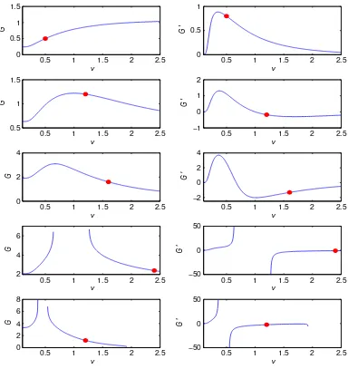
Because a thorough understanding of the function G(v) is crucial, we plot the function G(v) and its derivative in v in Figure 2 for five different parameter combinations (x, v∗, ω). For ease of exposition, we fix x =−0.5 and vary v∗ and ω. Figure 2 shows that all of the following five behavior of G(v) can occur, corresponding to the five rows of the subplots:
2. G(v) is globally well-defined, not globally contracting, but locally contracting around v∗. This corresponds to the second row of Figure2, where v∗ = 1.2 and ω= 0. 3. G(v) is globally well-defined, but not locally contracting around v∗. This
corre-sponds to the third row of Figure2, wherev∗ = 1.8,ω=−0.28, andG′(v∗)=. −1.32.
4. G(v) is not globally well-defined, but locally contracting around v∗. This
corre-sponds to the fourth row of Figure2, wherev∗ = 2.4, ω=−0.1, andG′(v∗)=. −0.89.
5. G(v) is not globally well-defined, and not locally contracting around v∗. This corresponds to the last row of Figure2, wherev∗= 1.2, ω=−0.66, andG′(v∗)=. −2.47.
In the rest of this section, we will analyze the global well-definedness property, local conver-gence properties, as well as the global converconver-gence properties of theSOR algorithm.
3.2. Global well-definedness property of the SOR algorithm
We will look at well-definedness first. It is extremely difficult to analyze local well-definedness for a fixed starting point v0. The following numerical example illustrates this point. Letx=−0.5, v∗ = 2.5 and ω =−0.1. Then G(v) is not defined forv ∈[0.548467,1.46434]. This means that
we cannot start theSOR algorithm from a point in this region. However, if v0 = 0.03, then the
sequence jumps past this bad region to v1 = 2.2285 and converges tov∗. Thus, in the following
we look for a global well-definedness condition which guarantees that the sequence vk is well-defined regardless of the initial point v0. We will focus on x < 0 since we show later that the
well-definedness property withx= 0 is quite simple to analyze even for a fixed starting pointv0. First we define a functionev=ev(w;x) as follows. For anyx≤0 and−1< ω <1, we let
e
v=ev(ω;x) =p2|x|
r 1 +ω
1−ω. (16)
We will often simply write ev orev(ω) forve(ω;x). We first establish two lemmas.
Lemma 3.2. Let x <0. Then, we havelimv→0+F(v) =c∗ and limv→+∞F(v) =c∗+ω. Also,
if ω ∈(−1,1), then F(v) strictly increases on (0,ev) and strictly decreases on(ev,∞). If ω ≥1, then F(v) strictly increases for all v >0.
Lemma 3.3. Let x <0. Suppose ω∈(−1,1). Define
H(ω) =H(ω;x, v∗)≡c∗+N−(ve(ω)) +ωN+(ve(ω))−(1 +ω). (17)
Then, H(ω) has a unique root ωb in (−1,1). Furthermore, if ω ≤ bω, then H(ω) ≥ 0, and if ω >ωb, then H(ω)<0.
The following theorem gives a necessary and sufficient condition for global well-definedness of the SORalgorithm when x <0. The x = 0 case is deferred to Theorem3.6 because a separate analysis is needed for this simpler case.
Theorem 3.1. (global well-definedness)Let x <0. Whenω ≥1, {vk} in theSORalgorithm
is well-defined for anyv0 ∈R+. When −1< ω <1, {vk}is well-defined for any v0∈R+ if and only if ω >ωb and ω≥ −c∗.
While the global well-definedness condition guarantees that the SOR algorithm produces a well-defined sequence, it does not guarantee that such an ω will make the SOR algorithm convergent. In the following, we study the local and global convergence properties of the SOR
algorithm.
3.3. Local convergence properties of the SOR algorithm
We will first analyze the local convergence properties. We say that theSORalgorithmconverges locallyif there exists a neighborhoodVǫ ofv∗, such that the for any v0∈Vǫ, the SORalgorithm converges. Let us introduce two functions Φ(v;x) and Ψ(v;x) defined as follows
Φ(v;x) = v
2−2|x|
v2+ 2|x|, and Ψ(v;x) =
−2|x|
v2+ 2|x|. (18)
We will write Φ(v) instead of Φ(v;x) unless we want to emphasize the dependence onx. Similarly for Ψ(v;x). The two functions are related through Φ(v) = 1 + 2Ψ(v). Notice that whenx <0,
−1 < Φ(v) < 1, −1 < Ψ(v) < 0, and both Φ(v) and Ψ(v) are strictly increasing in v. When
x = 0, Φ(v) ≡1 and Ψ(v) ≡0. These two functions Φ(v) and Ψ(v) play extremely important roles in the analysis that follows.
The following lemma gives properties of the iteration function G(v). In particular, it says that G(v) is strictly increasing on any connected open subsets of DomG∩ {v:ω >Φ(v)}.
Lemma 3.4. Let x≤0. Let DomG denote the open set of v for whichG(v) is well-defined in a neighborhood of v. For v ∈DomG, we have
dG(v)
dv =
ω−Φ(v) 1 +ω
G(v)2n+(v) v2n+(G(v))
v2+ 2|x|
G(v)2+ 2|x|. (19)
Furthermore, v∗∈DomG, and
G′(v∗) =
ω−Φ(v∗)
1 +ω . (20)
We need another technical lemma to establish the local convergence property. Define a new functionQ(v;x, v∗, ω) : DomG7→Ras follows:
Notice that Q(v∗) = 0. Suppose G(v) and G(G(v)) are both defined. Taking the sum of two
consecutive iteration equations, we have
Q(v) = (1 +ω)[N+(v)−N+(G(G(v))]. (22)
Thus, the sign of Q(vk) controls whether vk+2 is larger than vk or not. In particular, to help convergence, we would like to seeQ(v)>0 ifv > v∗andQ(v)<0 ifv < v∗. The following lemma gives the derivatives ofQ(v). It is useful in proving both Theorem3.2on local convergence and Theorem3.9 on global convergence.
Lemma 3.5. For any v∈DomG, the derivative of Q(v) is given by
Q′(v) = n
+(v) |x|
G(v)2 +12
·µ
|x| v2 +
|x| G(v)2
+ ω
1 +ω
¸
. (23)
In particular, when v=v∗, we have
Q′(v∗) =
2n+(v∗)
1 +ω
£
ω−Ψ(v∗)
¤
. (24)
Furthermore, when ω= Ψ(v∗), we haveQ′(v∗) =Q′′(v∗) = 0 and
Q′′′(v∗) =
2n+(v ∗)|x| v4
∗(v∗2+ 2|x|)
(12v∗2−v4∗+ 4x2).
The above two lemmas give the following theorem, which establishes conditions for theSOR
algorithm to have local convergence.
Theorem 3.2. (conditions for local convergence) Let ω >−1.
1) Whenx <0, a necessary condition for the SORalgorithm to converge locally isω ≥Ψ(v∗)
and a sufficient condition is ω > Ψ(v∗). If ω = Ψ(v∗), a further necessary condition for local convergence is 12v2∗−v∗4+ 4x2≥0 while a further sufficient condition is12v∗2−v4∗+ 4x2 >0.
2) When x = 0, the necessary and sufficient condition for the SOR algorithm to converge
locally isω >0.
Ordinarily, to check these conditions, we would need to know the value ofv∗, which is the goal
of theSORalgorithm. However, in the next section, we will introduce two acceleration techniques which employ the above theorem but avoid the knowledge of v∗. In one of the techniques, we
dynamically vary ω in each iteration k, such that ωk is eventually larger than Ψ(v∗). In the
other technique, we setωto be the constant 1 in each iteration soω≥Ψ(v∗) is trivially satisfied.
Although we give a detailed proof of Theorem 3.2 in the Appendix, Theorem 3.2 (except for the borderline case ω = Ψ(v∗)) is actually a special application of a well-known result in
when x <0, the condition ω >Ψ(v∗) is only sufficient but not necessary for local convergence,
and the conditionω ≥Ψ(v∗) is necessary but not sufficient. This is because the borderline case ω= Ψ(v∗) is a little bit complicated. TheSORalgorithm can either locally converge or diverge in
this case. When bothω = Ψ(v∗) and 12v∗2−v4∗+ 4x2 = 0 hold, it can be shown thatQ(4)(v∗) = 0
since in this case it is proportional to [3v∗6−6v4∗x+ 24x3−4v∗2x(8 + 3x)](12v2∗−v∗4+ 4x2).Thus, a further condition on Q(5)(v∗) is needed to guarantee local convergence. We do not analyze this double borderline case in more detail because we will never encounter it in our actual implementation.
The following function will play a pivotal role in the analysis of theSOR algorithm:
φ(u, v) =φ(u, v;x)≡
N−(u)−N−(v)
N+(v)−N+(u) ifu6=v,
Φ(u;x) ifu=v.
(25)
Lemma 3.6. The functionφ(u, v)is symmetric inuandvand continuous onR2+. Furthermore, ifx <0, then|φ(u, v)|<1, and for any fixedv,φ(u, v)is continuously differentiable and strictly increasing in u, with the derivative given by
φ1(u, v) =
n+(u)
[N+(u)−N+(v)]2
½
x
u2[c(u)−c(v)] +
1 2[c
+(u)−c+(v)]
¾
if u6=v,
4|x|v
(v2+ 2|x|)2 if u=v.
(26)
Similarly, for any fixed u,φ(u, v) is continuously differentiable and strictly increasing inv, with φ2(u, v) =φ1(v, u). If x= 0, then φ(u, v)≡1 on R2+.
The following three lemmas are useful in analyzing both the local and global behavior of the sequence {vk}from the SOR algorithm.
Lemma 3.7. Let {vk} be a well-defined SORsequence and vk 6=v∗ for allk∈N. 1) If vk< v∗, then vk+1 > vk;
2) If vk> v∗, then vk+1 < vk.
Lemma 3.8. Let {vk} be a well-defined SOR sequence and vk 6= v∗ for all k ∈ N. Then for any k, we haveω 6=φ(vk, v∗), and
1) If ω > φ(vk, v∗), then vk and vk+1 are on the same side of v∗; 2) If ω < φ(vk, v∗), then vk and vk+1 are on the opposite side of v∗.
Lemma 3.9. Let {vk} be a well-defined SORsequence and vk 6=v∗ for allk∈N. 1) If 1 + 2ω > φ(vk, vk+1), then vk+1 and vk+2 are on the same side of vk;
2) If 1 + 2ω < φ(vk, vk+1), then vk+1 and vk+2 are on the opposite side of vk;
The next theorem states that if the SOR algorithm converges, then it is either eventually monotone or eventually oscillating around v∗.
Theorem 3.3. (local convergence pattern) Let x ≤ 0. Suppose that vk from the SOR
algorithm converges to v∗ and vk 6= v∗ for all k ∈ N. Then there exists a k0 ∈ N, such that if k > k0, the following is true:
1) If ω≥Φ(v∗), then vk approaches v∗ monotonically;
2) If ω <Φ(v∗), then vk is oscillating around v∗. More specifically, for any m∈N, we have vk0+2m < vk0+2m+2 < v∗ and vk0+2m−1> vk0+2m+1> v∗.
We give two more results on the patterns of theSORalgorithm below.
Theorem 3.4. (local pattern for |ck−c∗|) Suppose that the SOR algorithm converges to v∗ with vk 6=v∗ for allk∈N. Then the sequence|ck−c∗|eventually monotonically decreases to 0.
Theorem 3.5. (local pattern for |vk−v∗|) Suppose that the SOR algorithm converges to v∗ and vk 6=v∗ for all k∈ N. When ω > Ψ(v∗), |vk−v∗| is eventually monotonically decreasing. When ω = Ψ(v∗),|vk−v∗|is eventually monotonically decreasing if and only ifv∗ =
p 2|x|.
Whenω = Ψ(v∗) andv∗ 6=
p
2|x|,|vk−v∗|no longer monotonically decreases to 0. However,
in this case, vk oscillates around v∗ and the two subsequences above and below v∗ approach v∗
monotonically.
3.4. Global convergence properties of the SOR algorithm
In the actual implementation it is hard to know whether the initial v0 is close enough tov∗ or not. Thus, in the following we study the global convergence properties. That is, in the analysis below, we do not assume that v0 is close to v∗. Furthermore, in the majority of the analysis below, we also do not assume that the global well-definedness condition is satisfied.
The following theorem completely characterizes the well-definedness and convergence pat-terns for the SOR algorithm when x = 0. Recall from Theorem 3.2 that a necessary condition for the algorithm to converge when x= 0 is ω >0.
Theorem 3.6. (SOR algorithm when x = 0) Assume x = 0 and v0 6= v∗. We have three
cases:
1) ω > 1. In this case, the SOR algorithm is globally well-defined and convergent.
Further-more, if v0 > v∗, then vk strictly decreases to v∗. If v0< v∗, then vk strictly increases to v∗. 2) ω = 1. In this case, the SOR algorithm is globally well-defined and convergent. In fact,
vk=v∗ for any k≥1.
3) 0< ω <1. In this case, the SOR algorithm is well-defined if and only if G(v0) is defined.
Furthermore, if G(v0) is defined, then the SOR algorithm is convergent and {vk} is immediately
The following analysis will focus on x < 0. We first consider the baseline case ω = 0 in the SORalgorithm. The following theorem shows that in this case, the SORalgorithm is always globally well-defined and convergent provided that v1 is defined.
Theorem 3.7. (SORalgorithm when ω = 0) Let x <0andω = 0. Supposec∗+N−(v0)<1, then {vk} in the SOR algorithm is globally well-defined and converges to v∗. Furthermore, the condition c∗ +N−(v0) < 1 is always satisfied when v∗ ≤
p
2|x|, and satisfied if v0 ≥ v∗ or v0 ≤2|x|/v∗ when v∗ >p2|x|.
We will now consider a general relaxation parameterω. Since a necessary condition for the
SORalgorithm to converge locally is ω≥Ψ(v∗), we only consider suchω’s.
It turns out that whenω ≥Φ(v∗), theSOR algorithm is globally convergent if the sequence
is well-defined. By Theorem 3.3, the SORsequence eventually monotonically approachesv∗ if it converges in this case.
Theorem 3.8. (SOR algorithm when ω ≥Φ(v∗)) Let x <0 and v0 6=v∗. Assume that ω ≥
Φ(v∗). When v0 < v∗, {vk} from the SOR algorithm is globally well-defined and monotonically
increases to v∗. When v0 > v∗, we have the following three cases:
1) If ω > φ(v0, v∗), then {vk} is globally well-defined and monotonically decreases to v∗. 2) If ω=φ(v0, v∗), then {vk} is globally well-defined and vk=v∗ for allk≥1.
3) If Φ(v∗)≤ω < φ(v0, v∗), then {vk} is globally well-defined if v1 is defined. Furthermore, if v1 is defined, then v1 < v∗ and the sequence monotonically increases to v∗.
While the above theorem completely characterizes the behavior of the SORalgorithm when
ω ≥Φ(v∗), we do not have a complete characterization for theω <Φ(v∗) case. Notice that by
Theorem3.3, theSORsequence is eventually oscillating aroundv∗if it converges whenω <Φ(v∗).
Nevertheless, we have obtained three sufficient conditions to guarantee convergence that are possibly weaker than ω ≥ Φ(v∗). These are given in the three theorems that follow. They
show that to have global convergence, we only need to slightly strengthen the local convergence condition ω≥Ψ(v∗), which is the same as 1 + 2ω≥Φ(v∗).
Theorem 3.9. (first sufficient condition for global convergence)Letx <0. Suppose that ω ≥Ψ(√2v∗). Let {vk} be the SOR sequence, possibly only defined for finitely many k. Let vk0
be well-defined and the first point in the sequence {vk} such that ω < φ(vk, v∗). Then the whole sequence {vk} is well-defined if and only if G(vk0) is defined. Furthermore, ifG(vk0) is defined,
then the SORalgorithm converges to v∗.
Theorem 3.10. (second sufficient condition for global convergence)Let x≤0. Suppose that theSORsequence{vk}is well-defined and bounded above by somev≥v∗. Then the sequence
converges to v∗ if 1 + 2ω > φ(v∗, v).
For the last theorem, we first need to establish some properties ofφ(u, G(u)).
Lemma 3.10. Let x <0, −1< ω <1, and u∈DomG. If u < G(u), there exists K >0, such that
φ(u, G(u))′ > K(ω−Φ(u)).
As a result, when ω < Φ(v∗), we have φ(u, G(u))′ > 0 if u < ve, where ev is the unique point satisfying ω= Φ(ev).
Theorem 3.11. (third sufficient condition for global convergence) Let x ≤0. Suppose
that ω satisfies the global well-definedness condition. Then for any v0 ∈R+, theSOR algorithm
converges to v∗ if
1 + 2ω > sup
e
v<u<v∗
φ(u, G(u)). (27)
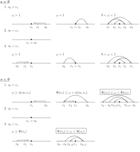
Figure3summarizes the results of this section by giving all the possible convergence patterns for theSORalgorithm. The top half of Figure3plots all the possible convergence patterns when
x= 0. Notice that by Theorem3.6all the conditions above each subplot are both sufficient and necessary for that particular convergence pattern to occur. The bottom half of Figure 3 plots all the possible convergence patterns when x < 0. Notice that Theorem 3.8 only guarantees convergence when ω ≥ Φ(v∗). We box two conditions in two of the subplots to indicate that
these conditions are only necessary and not sufficient for these two particular global convergence patterns.
4. Convergence acceleration methods
4.1. The convergence order of the SOR algorithm
We next take a look at the speed of convergence. We make use of the following common notions of convergence speed. Suppose that the sequencevk converges tov∗. We say that this sequence
converges linearly if there exists a numberµ∈(0,1) such that
lim k→+∞
|vk+1−v∗|
|vk−v∗|
=µ. (28)
rate. A smaller µmeans faster convergence. We say that the sequence converges with orderq if for someq ∈N,
lim k→+∞
|vk+1−v∗|
|vk−v∗|q
=µwith µ >0. (29)
In particular, convergence with order 2 is called quadratic convergence. The following proposi-tion shows that theSOR algorithm in the last section usually has a linear order of convergence.
Theorem 4.1. (convergence order of theSOR algorithm)Let x≤0. Suppose thatvk from
the SOR algorithm converges to v∗ and vk6=v∗ for all k∈N. Then,
1) If ω6= Φ(v∗) and ω >Ψ(v∗), the sequence {vk} has a a linear order of convergence, with
convergence rate µ=|G′(v∗)|.
2) If ω= Φ(v∗), then the sequence converge superlinearly. 3) If ω= Ψ(v∗), then the sequence converges sublinearly.
The above theorem immediately implies the following. Consider a fixed option with money-nessx≤0 and implied volatilityv∗. LetvkAandvkBbe two convergent SORsequences associated with initial values v0A and vB0, and relaxation parameters ωA and ωB, respectively. Suppose
vi
k 6=v∗ for all k ∈ N, i= A, B. If µA < µB, then Theorem4.1 implies that regardless of the relative accuracy ofvA
0 andv0B, there existsk0 ∈N, such that for allk > k0,|vkA−v∗|<|vkB−v∗|. Thus, in selecting ω, we should try to select it such that it is as close to Φ(v∗) as possible. In
particular, ifω happens to be Φ(v∗), then we have superlinear convergence.
A linear convergence order is not very efficient. The rest of this section improves the con-vergence order of the SORalgorithm through two convergence acceleration techniques: dynamic relaxation and transformation of sequence.
4.2. Dynamic relaxation (SOR-DR)
Although the theory tells us that we should select ω to be Φ(v∗), in practice we do not know
the value of v∗, because after all, the precise value of v∗ is the goal of the SOR algorithm.
This difficulty can be overcome by a dynamic relaxation technique which approximates Φ(v∗)
adaptively with Φ(vk). More specifically, we modify theSOR algorithm to the following, which we label as the SOR-DRalgorithm.
1. Select an initial point v0 and set ω0 = Φ(v0);
2. (SOR-DR) After obtaining vk, compute vk+1 from the following equation
vk+1=G(vk;x, v∗, ωk), (30)
and set ωk+1 = Φ(vk+1);
3. Stop when |vk−v∗|< ǫ or |ck−c∗|< ǫ, for some ǫ small.
Theorem 4.2. (convergence properties of theSOR-DRalgorithm)Whenx= 0, theSOR-DR
algorithm is globally well-defined and vk = v∗ for all k ∈ N. When x < 0 and v0 > v∗, vk is globally well-defined and monotonically decreases to v∗. When x < 0 and v0 < v∗, the
SOR-DR algorithm is globally well-defined if v1 is defined. If v1 is defined, then v1 > v∗, and vk
monotonically decreases to v∗ afterwards.
In addition to having nice global well-definedness and convergence properties, the SOR-DR
algorithm has at least quadratic order of convergence.
Theorem 4.3. (convergence order of the SOR-DR algorithm) Assuming vk6=v∗ for all k,
the SOR-DR algorithm has at least a quadratic order of convergence if v1 is defined.
Theorem4.3is a very interesting result, because while the Newton-Raphson algorithm uses derivative information of c(x, v), the SOR-DR algorithm never requires the calculation of the derivatives. The derivative of c(x, v) with respect to v is given by n+(v). For deeply away-from-the-money options, n+(v) could be extremely small, often resulting in overflow problems in implementing the Newton-Raphson algorithm. That the SOR-DR algorithm works well for away-from-the-money options is one major advantage over the Newton-Raphson method.
4.3. Transformation of sequence (SOR-TS)
While we can obtain quadratic order of convergence through a dynamic relaxation technique, quadratic convergence can also be obtained through a classical transformation of sequence tech-nique. Well-known examples of sequence transformation include Aitken’s delta-squared method and Richardson extrapolation. A very good up-to-date reference to this technique is Sidi (2002). We will label the following theSOR-TSalgorithm.
1. Select an initial point v0 and a relaxation parameter ω;
2. (SOR-TS) After obtaining vk, compute vk+1 from the following equation
vk+1=αkG(vk;x, v∗, ω) + (1−αk)vk, (31)
where
αk=
1 +ω
1 + Φ(vk); (32)
3. Stop when |vk−v∗|< ǫ or |ck−c∗|< ǫ, for some ǫ small.
The iteration step in theSOR-TSalgorithm can be more succinctly written as
vk+1=M(vk;x, v∗, ω), (33)
where the iteration functionM(v;x, v∗, ω) is given by
M(v) =M(v;x, v∗, ω)≡
1 +ω
1 + Φ(v;x)G(v;x, v∗, ω) + µ
1− 1 +ω 1 + Φ(v;x)
We will use the common practice in numerical analysis of using the term extrapolation generally to include interpolation. That is, we treat extrapolation as a synonym for sequence transformation. The transformation of sequence technique above is a simple extrapolation using only two points vk and G(vk). The weight αk is chosen carefully so that M′(v∗;x, v∗, ω) = 0,
which guarantees at least quadratic order of convergence if the SOR-TS algorithm converges. Using the notions in Sidi (2002), the extrapolation is nonlinear, in that the parameter αk is not a constant, but rather depends on the sequence {vk} itself. As Sidi (2002) points out, nonlinear extrapolation is usually needed to improve order of convergence. Also, the sequence transformation is iterative in that for each k, the extrapolated value vk is used to perform the next extrapolation to getvk+1.
Whileωis a free parameter in theSOR-TSalgorithm, there is some guidance on how to choose a goodω. First,ωshould be chosen such that the sequence{vk}is well-defined. Thus,ωcan not be too small. For example, ifω is close to Ψ(v∗),G(v) fails to be globally well-defined. Also, ω
can not be too large because a too largeω might send the extrapolated pointvk+1 below 0. The
following numerical example illustrates this point. Letx=−0.1,v∗= 0.1 andω= 5. Letv0 = 2.
Then G(v0) = 1.3137 and the extrapolated point v1 =−0.1617<0. Another consideration in
selecting ω is stability. Let bvk be the computed numerical value for vk. As Sidi (2002) points out, whenvk is sufficiently close tov∗, the round-off error|bvk−vk|might start to dominate the total error|vbk−v∗|. Furthermore, the round-off error might propagate and make the algorithm unstable if more than necessary many iterations are performed. There are a few possible sources of round-off errors. The first source is the iteration equation. This is due to the inaccuracy in computing the cumulative normal distribution and its inverse, and the effect is largely controlled by the coefficientsω and 1 +ω. For example, a very largeωwill amplify the errors. This source of round-off error is also present in the SOR-DRalgorithm. However, the SOR-TSalgorithm has another source of round-off error coming from the sequence transformation. The magnitude of this source is largely controlled by the coefficients αk and 1−αk.
Because of the above considerations, we recommend setting ω = 1 always in the SOR-TS
algorithm. There are several reasons for this choice. First, the choice of ω = 1 is good from stability considerations. Second, if x = 0 and ω = 1, we immediately have G(v1) = v∗, and
sinceα1= 1, we have v1=v∗. That is, the sequence immediately lands onv∗. Finally, if x <0 and ω= 1, Theorem3.1guarantees the global well-definedness ofG(v), and Theorem4.4below in turn guarantees the global well-definedness ofM(v). The global well-definedness property is extremely useful because it brings in the robustness of theSOR-TSalgorithm.
We first establish some useful results for the extrapolated iteration function M(v;x, v∗, ω)
in Lemma 4.1below whenω= 1. These results will be used in Theorem 4.4.
Lemma 4.1. Let x <0 and ω= 1. The derivative ofM(v) with respect tov is given by
M′(v) =−4G|x|
v3 +
2|x| v2 +
n+(v)
n+(G)
1
1 2 +
|x|
G2
µ
|x| v2 +
2x2 v4
where we have written G for G(v;x, v∗,1). Furthermore, M(v) > 0 for all v ∈ R+. Also, we have M′(v∗) = 0, and
M′′(v∗) =− | x|
2v3
∗(v2∗+ 2|x|)2
m(v∗, x)
where the function m(v, x) is given by m(v, x) =v6−2(4 +x)v4−4x2v2+ 8x3. For any fixed x <0, there exists a unique vr=vr(x)∈R+ such that m(vr, x) = 0. Furthermore,m(v, x)<0
when v < vr, and m(v, x)>0 when v > vr.
SinceM′(v∗) = 0, we immediately have local convergence. Also, the sign ofM′′(v∗) controls the convergence pattern. For global convergence, we need to define two more quantities:
Mmin(x, v∗)≡inf{M(v;x, v∗,1) :v≥v∗}, (36) B(x, v∗)≡sup{|M′(v;x, v∗,1)|:v≥Mmin(x, v∗)}. (37)
Notice that since M(v∗) =v∗, we have Mmin(x, v∗)≤v∗. We have the following theorem:
Theorem 4.4. (convergence properties of the SOR-TS algorithm) Let x ≤ 0. Then the
SOR-TS algorithm with ω = 1 is globally well-defined and {vk} converges to v∗ locally. For any
option with (x, v∗), the SOR-TS algorithm converges globally for any v0 ∈ R+ if B(x, v∗) < 1. Furthermore, if x = 0, then vk = v∗ for all k ∈ N. If x < 0 and {vk} converges to v∗ with vk6=v∗ for all k∈N, we have
1) The sequence{vk} eventually decreases to v∗ if v∗ < vr(x). 2) The sequence{vk} eventually increases to v∗ if v∗> vr(x).
3) Ifv∗ =vr(x), the convergence can be either eventually monotone or eventually oscillating.
The condition B(x, v∗) < 1 is only sufficient for global convergence and not necessary.
Through extensive numerical analysis, we conjecture that the SOR-TSsequence converges glob-ally without this condition, but so far we are not able to prove it analyticglob-ally. In any case, we have numerically verified (details are available upon request) that the conditionB(x, v∗)<1 is
satisfied inside a very large domain D− on which we will implement our algorithms. That is, inside the domain D−, theSOR-TSalgorithm with ω= 1 is globally convergent.
Theorem 4.5. (convergence order of the SOR-TS algorithm) Let x ≤ 0. Assuming the
sequence{vk} from theSOR-TSalgorithm withω= 1 converges to v∗ withvk6=v∗ for all k∈N, then the sequence has at least a quadratic order of convergence.
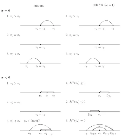
Figure 4 gives all the convergence patterns for theSOR-DR and SOR-TS(ω = 1) algorithms. Notice that the two algorithms are always globally well-defined, except that when v0 < v∗
eventually converges tov∗ monotonically from above. We classify the local convergence behavior
of the SOR-TSalgorithm according to the sign of M′′(v∗). The three conditions listed should be
interpreted as necessary conditions. For example, a necessary condition for theSOR-TSsequence to eventually decreases tov∗ is that M′′(v∗)≥0.
While the above discussion has focused on improving the asymptotic convergence speed of the SOR algorithm by modifying the iteration step, in the actual implementation the initial estimate v0 is often of crucial importance because in practice only a finite number of iterations can be performed. A good estimate v0 usually also helps with numerical stability. Therefore, for each option with observed moneynessxand option pricec∗, we use a rational approximation v0 =v0(x, c∗) for the initial estimate. This will be discussed in detail in the next section.
5. Numerical implementation and performance
5.1. Numerical implementation with rational approximation enhancement
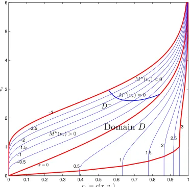
First, we will describe the domain of inversion. The domain of inversion consists of all options we consider, with different values of moneyness x and implied total volatility v∗. We will restrict v∗ ≥0.0005 since volatilities lower than this bound are extremely rare in real financial applications. Options with values c∗ extremely close to 0 or 1 are also excluded. The final inversion domainD we consider is as follows:
D={ |x| ≤3, 0.0005≤v∗≤6, 0.0005≤c∗ ≤0.9995, |x|/v∗≤3}. (38)
Notice that this domain is much larger than those considered by most authors. For example, in Li (2008),v∗ is bounded above by 1,|x|bounded by 0.5, andx/|v∗|bounded by 2. Figure5
plots the domain D in the two-dimensional (c∗, v∗)-space. Recall that we will only consider
options with x ≤ 0 by the “in-and-out” duality. We denote the left half of D by D−, where
x≤0. Notice we have also plotted the curveM′′(v∗) = 0, which is the same asv∗ =vr(x). By
Lemma 4.1, this curve separates the left domainD− further into two parts.
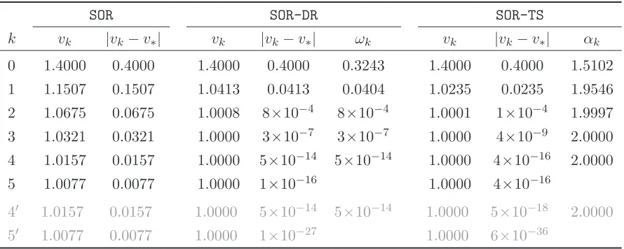
Before we look at theSOR-DR and SOR-TSalgorithms in the whole domain D−, let us look at their performance on a particular option. The option used has moneyness x = −0.5 and volatility v∗ = 1. For the SOR and SOR-TS algorithms, we set ω = 1 for all the iterations.
Table 1 shows the effect of introducing dynamic relaxation or sequence transformation to the
SOR algorithm. All the numbers are computed using Mathematica 6.0 with (10−16)-precision
arithmetic, except for the rows labeled as 4′ and 5′, where all the numbers are computed with
(10−50)-precision arithmetic. For all three algorithms, the initial estimate v0 is set to be 0.6
in Panel A and 1.4 in Panel B. While all three algorithms converge to the true v∗, the SOR-DR
and SOR-TSalgorithms converge much faster. In each of the two latter algorithms, the number of correct digits roughly double after each iteration, indicating quadratic convergence. For the
Φ(v∗) = 0 quickly, giving rise to quadratic convergence. For the SOR-TSalgorithm, we also give
the value ofαk for each iteration. As we see,αk approaches a value of 2 quickly. Thus for each iteration, after getting G(vk), the SOR-TSalgorithm will perform an extrapolation, which is the source of the quadratic convergence. Also notice that the round-off error kicks in and dominates the total error whenvk is extremely close to v∗ if we use (10−16)-precision arithmetic.
We now consider the choice of v0 =v0(x, c∗). For each option characterized by (x, c∗), we use the following third-order rational approximation for the initial estimate v0:
v0=
P
i+j≤3mij xicj∗
P
i+j≤3nij xicj∗
, (39)
where mij and nij are coefficients and we set n00 = 1 for normalization. Thus there are a
total of 19 parameters. We search for the optimal values for {mij} and {nij} numerically by minimizing the uniform error in v∗ from both theSOR-DR and SOR-TSalgorithms. Specifically,
let vSOR-DR
k and v
SOR-TS
k denote the numerical estimate of v∗ after k iterations for a fixed set of parameters{mij}and{nij}from theSOR-DRandSOR-TSalgorithms, respectively. Our objective is to search for the optimal parameters through the following problem:
GD = min
{mij},{nij}
max
(x,v∗)∈D−
g(x, v∗,{mij},{nij}), (40)
whereg is the error function for each fixed option (x, v∗) with parameters{mij}and {nij}:
g(x, v∗,{mij},{nij}) = ¯ ¯vSOR-DR
k −v∗
¯
¯+¯¯vSOR-TS
k −v∗
¯ ¯.
We have set k to be the same for all options in domain D− for vectorization consideration. Vectorization increases the efficiency of our algorithms. To compute the max part of the above objective function, we populate the domain D− densely with roughly one million options, with the boundary populated denser than the inner region. Each of these options is characterized by a different pair of value (x, v∗). For each fixed set of parameters{mij} and {nij}, we compute
vSOR-DR
k and v
SOR-TS
k , and then approximate the uniform error with the maximum error in v∗ of all the options. If the domain D− is populated sufficiently densely, this is a very accurate
approximation. For the min part, we use a downhill simplex method of Nelder and Mead (1965), which is described in detail in Press et al. (1992). The choice of using the simplex method is dictated by the fact that we do not have any derivative information of the objective function with respect to the parameters{mij}and {nij}.
A few details are worth brief mentioning. First, it is extremely difficult to minimize over uniform errors using simplex methods because uniform errors are prone to problems such as local minimums, slow convergence, etc. Thus, we actually minimize the following penalized objective function
GDλ = min
{mij},{nij}
µ max
(x,v∗)∈D−
g(x, v∗,{mij},{nij}) +λ X
(x,v∗)∈D−
g(x, v∗,{mij},{nij}) 
where λ controls the strength of penalty. When λ is larger, the objective function becomes smoother but deviates more from the uniform error. We dynamically adjust the value λ so that we put more weight on the uniform error as we move closer to the optimal values for
{mij} and {nij}. Second, we set k = 5. Numerically, we find that setting k = 5 uniformly for all options achieves the best combination of accuracy and efficiency. Finally, by design, the rational approximation estimatev0 is not necessarily close to v∗ for a given option (x, v∗). This is becausevk in our algorithms can “jump” and globally it is not always the case that a closerv0 would result in a quicker convergence tov∗.
Our final choice for the{mij} and{nij} from the above numerical procedure is:
m00=−0.00006103098165; n00= 1;
m01= 5.33967643357688; n01= 22.96302109010794;
m10=−0.40661990365427; n10=−0.48466536361620; m02= 3.25023425332360; n02=−0.77268824532468; m11=−36.19405221599028; n11=−1.34102279982050;
m20= 0.08975394404851; n20= 0.43027619553168; (42) m03= 83.84593224417796; n03=−5.70531500645109;
m12= 41.21772632732834; n12= 2.45782574294244; m21= 3.83815885394565; n21=−0.04763802358853; m30=−0.21619763215668; n30=−0.03326944290044.
Plugging the above parameters values into equation (39) gives us the initial starting point v0
for the successive over-relaxation algorithms.
5.2. Numerical performance
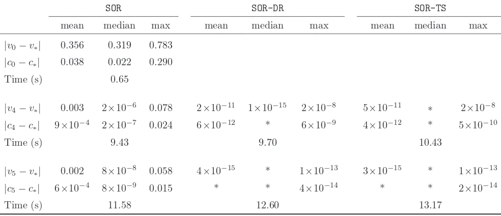
Table2gives the performance of the three algorithmsSOR,SOR-DR,SOR-TSinside the domainD−. The accuracy is measured in terms of both |vk−v∗|and |ck−c∗|. All three algorithms are
im-plemented with (10−16)-precision arithmetic in MATLAB 7.1 on a Dell Dimension 4600 desktop
computer (2.8 GHz, 1G RAM). We report the accuracy of the rational approximation (k= 0), and of each of the three algorithms whenk= 4 andk= 5. The means, medians and maximums of |vk−v∗| and |ck−c∗| are calculated by uniformly and densely populating the domain D−
with roughly 1 million options. The computing time for all options of each algorithm is also reported fork= 0,4 and 5. As we see, the rational approximation has a uniform error of 0.783 for|vk−v∗|and a uniform error of 0.29 for |ck−c∗|in domainD−. Thus, the rational
takes only 0.65 seconds for all roughly one million options. When k = 4, both the accelerated algorithmsSOR-DR and SOR-TSachieve a uniform error in v∗ in the order of 10−8 while that of
the SORalgorithm is 0.078. The medians of the errors in v∗ and c∗ are quite small for all three
algorithms. The larger errors tend to occur near the boundary of the domain D−. All three algorithms take around 12 seconds. Fork= 5, both accelerated algorithmsSOR-DRand SOR-TS
achieve a uniform error in v∗ in the order of 10−13 while that of the SOR algorithm is 0.058. We do not recommend using more than 5 iterations because the round-off error can start to dominate the total error in v∗. The computing times are still only about 12 seconds for all
roughly one million options. Overall, we see that the performance of the SOR-DR and SOR-TS
algorithms are quite good in terms of both accuracy and speed. Also, numerically we find that our algorithms work for a much larger domain with only a slight decrease in accuracy.
Most existing methods fail to work in our large domainD−. This is the case, for example, for
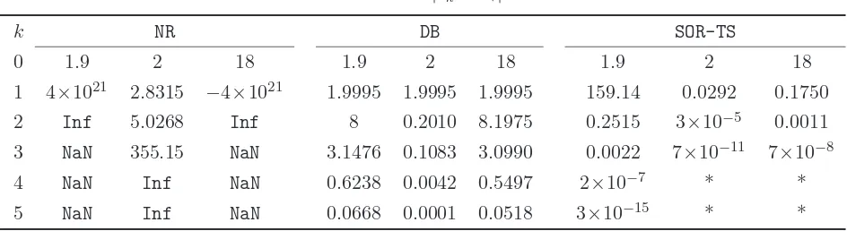
the Corrado-Miller method and the rational approximation of Li (2008). Thus we cannot perform a comparison between these methods and ours. One exception is the Dekker-Brent algorithm. Table3compares the performance of theSOR-TSalgorithm, the Newton-Raphson algorithm, and the Dekker-Brent algorithm for a particular option (x, v∗), where we letx=−1 andv∗ = 2. We
do not consider theSOR-DRalgorithm in this comparison, because its performance is very similar to that of the SOR-TS algorithm, except for the fact that the SOR-DR algorithm is not always globally well-defined. We start all three algorithms from three different initial values, namely, 0.1, 4, and 20 and report the first 5 iterations (Panel A) together with the errors (Panel B). As we see, a naive implementation of the Newton-Raphson algorithm fails in all three cases. The reason is that in each Newton-Raphson iteration, one needs to divide the price error by the vega in each step. For away-from-the-money options, vega can be extremely small, leading to numerical instability. Although not reported, for this particular option, if we start from the the guess v0 =
p
2|x|as was suggested in Manaster and Koehler (1982), then the Newton-Raphson algorithm converges. However, examples can be easily given where even this choice ofv0=
p 2|x|
leads to failure in the Newton-Raphson algorithm. This happens for large values of |x|and v∗
in our domainD−. On the other hand, both theSOR-TSand Dekker-Brent algorithms converge in all three cases. The quadratic order of convergence of the SOR-TSalgorithm is evident after only one or two iterations. The Dekker-Brent algorithm uses a combination of bisection and interpolation and some of the bisection steps are evident in the table. Overall, the SOR-TS
algorithm achieves the best combination of robustness, efficiency and accuracy. One particular attractive feature of this algorithm is that it is globally convergent for any positivev0.
6. Further Applications
In the second example, we consider the implied volatility for call options in the Bachelier model. The last example considers the critical stock price level in a compound call on call option.
6.1. The Margrabe implied correlation
The most commonly used formula for the price of an exchange option is the Margrabe formula, which was independently discovered by Fischer (1978) and Margrabe (1978). Margrabe (1978) considers the price of an option to exchange one asset for another, while Fischer (1978) considers the price of a call option when the exercise price is uncertain.
Under the Margrabe formula setup, the dynamics of the two stock prices S1(t) and S2(t)
under the risk-neutral measureQ are given by
dSi(t) = (r−δi)Si(t)dt+σiSi(t)dWi(t), (i= 1,2)
where the two Brownian motions W1(t) and W2(t) are correlated with constant coefficient ρ.
The Margrabe formula gives the time-0 price C of a European option to exchange stock 2 for stock 1 at timeT as follows:
C =S1(0)e−δ1TN(d1)−S2(0)e−δ2TN(d2),
where
d1 = log[(S1(0)e
−δ1T)/(S
2(0)e−δ2T)] +σ2T /2
σ√T , d2 =d1−σ
√
T ,
and σ≡pσ2
1+σ22−2ρσ1σ2. Li (2007) contains three different methods to prove the Margrabe
formula.
In practice, people often use the Margrabe formula to compute the implied correlation ρ
from the observed option price C, with σ1 and σ2 estimated using some other methods. Our
methods can be applied directly to compute the implied correlation. This is because if we define
c=C/(S1e−δ1T), x= log[(S1(0)e−δ1T)/(S2(0)e−δ2T)], v=σ
√
T , (43)
then the Margrabe formula reduces to the dimensionless Black-Scholes formula in (1). The parameterv can then be computed using either theSOR-DRor theSOR-TSalgorithm. Once v is computed, the implied correlation can be computed by
ρ= σ
2
1T+σ22T −v2
2σ1σ2T . (44)
6.2. The Bachelier implied volatility
mathematically. Schachermayer and Teichmann (2007) contain an interesting comparison of Bachelier’s formula with that of Black and Scholes. The original Bachelier formula considers interest rater = 0. There are a few approaches to extend it to nonzero interest rates. We adopt the following one which models the risk-neutral dynamics of the stock price process as:
dSt=rStdt+σe(r−δ)tdWt.
Notice that we have introduced a nonzero dividend rate δ too. In this case, ST has the explicit solutionST =e(r−δ)T(S0+σWT),and the Bachelier formula for the time-0 price of a call option is given by
C=σ√T e−δTn(d) + (S0e−δT −Ke−rT)N(d), (45)
where
d= S0e
−δT −Ke−rT
σ√T e−δT .
In practice, people observe the actual price C∗ and compute the volatility parameter σ∗ which
satisfies the Bachelier formula. This parameter (after sometimes normalizing it byS0) is called the Bachelier implied volatility. It is also often called the normal volatility by practitioners because future stock price is assumed to be normally distributed in the Bachelier model.
Recently, Choi, Kim and Kwak (2007) develop a closed-form numerical approximation for the Bachelier implied volatility, which is found to be very accurate. In this paper, we will apply our successive over-relaxation method to compute the Bachelier implied volatility. We first make the following parameter reduction. Define the normalized call pricec, moneynessxand volatility
v as follows:
c=C/(S0e−δT), x= 1−
Ke−rT
S0e−δT
, v=σ√T /S0. (46)
Then Bachelier’s formula in equation (45) reduces to the following dimensionless Bachelier’s formula
c=cB(x, v) =v n(x/v) +xN(x/v). (47)
Notice that like the Black-Scholes formula, the Bachelier option price is also a strictly increasing function of v because the Bachelier vega is given by∂cB(x, v)/∂v=n(x/v)>0.
Like the dimensionless Black-Scholes formula, we only need to consider call options because put-call parity is also satisfied in the Bachelier framework. Also, we only need to consider out-of-the-money call options because of the following “in-out” duality in the Bachelier formula:
That is, to compute the Bachelier implied volatility for an option with positive moneynessxand normalized pricec∗, we could just compute the volatility for its dual option with moneyness−x
and normalized option price c∗−x.
Letv∗ be the true Bachelier implied volatility. That is, c∗ =cB(x, v∗). Define the iteration
functionGB(v;x, v
∗, ω) as follows:
GB(v;x, v∗, ω) =
c∗−xN(x/v) +ωvn(x/v)
(1 +ω)n(x/v) . (48)
We will sometimes just write GB(v). One possible successive over-relaxation method is the following, which we label as the SOR-Balgorithm:
1. Select an initial point v0;
2. (SOR-B) After obtaining vk, select ωk and compute vk+1 by
vk+1 =GB(vk;x, v∗, ωk), (49)
3. Stop when |vk−v∗|< ǫ or |ck−c∗|< ǫ, for some ǫ small.
It turns out that with the choice ωk = 0, the SOR-B algorithm is globally well-defined and converges tov∗ with a quadratic order of convergence.
Theorem 6.1. (convergence properties of the SOR-Balgorithm)Let ωk ≡0in the SOR-B
algorithm. Then the sequence{vk} is globally well-defined. If x= 0, then vk=v∗ for all k≥1. If x < 0 and v0 6= v∗, then v1 > v∗ and vk monotonically decreases to v∗ afterwards with a
quadratic order of convergence.
The efficiency of the SOR-B algorithm can be improved by introducing a rational approxi-mation like the one we did for the Black-Scholes implied volatility case. We omit the details here. Another way to extend the Bachelier model to nonzero interest rate is to model the stock price process as dSt= (r−δ)Stdt+σdWt.In this case, a different formula from equation (45) will be obtained. See, Musiela and Rutkowski (2005). However, our method of using successive over-relaxation to compute the Bachelier implied volatility is still applicable after some minor modifications.
6.3. The critical stock price in a compound option
Let the current date be 0, and T1 and T2 be two future dates with T2 > T1 >0. We will
let τ =T2−T1. Let the current stock price be S0, the constant interest rate ber, the dividend
rate be δ, and the volatility of the stock be σ. At timeT1, the holder of the compound option
is entitled to receive either cashK1, or a call option with strike priceK2 and maturity dateT2.
The time-0 value Cc of the compound option is given by
Cc=S0e−qT2N2(a1, b1;
p
T1/T2)−K2e−rT2N2(a2, b2;
p
T1/T2)−e−rT1K1N(a2),
whereN2(·,·;ρ) is the cumulative bivariate normal distribution function with correlationρ, and
a1=
log(S0/S∗) + (r−q+σ2/2)T1 σ√T1
, a2 =a1−σ
p
T1,
b1=
log(S0/K2) + (r−q+σ2/2)T2 σ√T2
, b2 =b1−σ
p
T2.
The formula for Cc is in closed form except that the critical stock price level S
∗ at time T1 to
exercise the compound option is given implicitly by
K1 =S∗e−qτN
µ 1
σ√τ log
S∗e−qτ K2e−rτ +
σ√τ
2 
−K2e−rτN
µ 1
σ√τ log
S∗e−qτ K2e−rτ −
σ√τ
2 
.
A Newton-Raphson algorithm can be used to computeS∗, but it is subject to the same numerical
instability we encountered before. To implement a successive over-relaxation method, we first perform a dimension reduction. Defining modified strikeκ, moneynessx, and total volatilityvby
κ= K1
K2e−rτ, x= log
S∗e−qτ
K2e−rτ, v=σ
√
τ , (50)
the critical stock price equation becomes
κ=κ(x, v) =exN(x/v+v/2)−N(x/v−v/2). (51)
The problem is then to compute the moneynessx∗that satisfies the above equation with observed modified strike κ∗ and assumed value of the total volatilityv.
Notice thatκ∗=κ(x∗, v). Define the iteration functionGCS(x;v, x∗, ω) by
GCS(x;v, x∗, ω) = log
µ
κ(x∗, v) +N(x/v−v/2) +ωexN(x/v+v/2)
(1 +ω)N(x/v+v/2)
. (52)
One possible successive over-relaxation method is the followingSOR-CSalgorithm:
1. Select an initial point x0;
2. (SOR-CS) After obtaining xk, select ωk and compute xk+1 by
xk+1=GCS(xk;v, x∗, ωk); (53)